GraphRAG: A Practitioner's Guide to 6 Advanced Architectural Patterns
A practitioner's look at six GraphRAG architectural patterns for production and what each one trades off in latency, cost and data freshness.
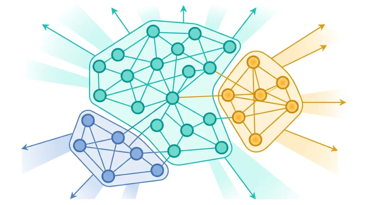
Enterprise knowledge‑intensive applications are increasingly expected to answer nuanced queries over massive, semi‑structured corpora while preserving latency budgets comparable to traditional search. Graph‑augmented Retrieval‑Augmented Generation (GraphRAG) promises to fuse the relational reasoning of graph databases with the generative power of large language models (LLMs), but the operational stakes-data freshness, cost predictability, and failure isolation-are amplified in production.
Context & Stakes
At its core, GraphRAG replaces the flat vector store of classic RAG pipelines with a property graph whose vertices encode document fragments, entity mentions, and LLM‑generated embeddings, while edges capture semantic relations such as co‑reference, hierarchical taxonomy, or temporal precedence. This structure enables multi‑hop traversal during retrieval, allowing a downstream LLM to receive a context that reflects both lexical similarity and logical connectivity. In practice, the graph is materialized in a purpose‑built engine (e.g., Neo4j, Amazon Neptune, or PostgreSQL with the Apache AGE extension) and kept in sync with a streaming ingestion pipeline that continuously extracts entities from new documents.
From a DevOps perspective, the shift from a single‑node vector index to a distributed graph service introduces three intertwined risk dimensions:
- Consistency latency. Graph updates must propagate across shards before they become queryable, otherwise the LLM may hallucinate based on stale relations. Systems that rely on eventual consistency (e.g., reads served from replicas) can exhibit a write-to-read window, which is unacceptable for real‑time chat assistants that promise sub‑second responses.
- Compute‑cost elasticity. Multi‑hop traversals are CPU‑intensive; each query may trigger a breadth‑first search across thousands of nodes, inflating per‑request cost relative to a single‑vector lookup. Without careful throttling, a traffic spike can exhaust CPU quotas, leading to cascading timeouts in downstream LLM calls.
- Observability complexity. Traditional RAG pipelines expose a single latency metric (vector similarity lookup). GraphRAG adds at least three additional dimensions-traversal depth, edge‑filter selectivity, and subgraph materialization time-each of which must be instrumented, correlated, and visualized to detect performance regressions.
Understanding these stakes requires a concrete example. Consider a financial services chatbot that ingests daily market reports, regulatory filings, and analyst notes. Each document is split into 200‑word chunks; entities such as ticker symbols, regulatory bodies, and macro‑economic indicators are extracted using a named‑entity recognizer (e.g., spaCy). The ingestion pipeline then creates vertices for each chunk and additional vertices for each entity, linking them with MENTIONS edges. A user asks, “How did the Fed’s policy change affect TechCorp’s stock over the last quarter?” The retrieval component must:
- Locate the
Fedentity node. - Traverse
POLICY_CHANGEedges to find associatedRegulationnodes dated within the last 90 days. - Follow
IMPACTSedges toTechCorpand finally to the relevantStockPricechunk vertices. - Aggregate the selected chunks into a prompt for the LLM.
Each hop adds latency; a naïve traversal that expands all neighbors can explode combinatorially, especially when high‑degree nodes like Fed have thousands of outgoing edges. Production teams therefore impose hard limits on traversal depth (typically 3 hops) and edge cardinality (e.g., cap at 500 neighbors per node). These limits are encoded directly in the query, through a bounded variable-length range and a result LIMIT, as illustrated below.
// Parameters: $fed = 'Federal Reserve', $ticker = 'TC'
MATCH (f:Entity {name: $fed})-[:POLICY_CHANGE*1..3]->(e)
WHERE e.date > date() - duration({days: 90})
MATCH (e)-[:IMPACTS]->(c:Company {symbol: $ticker})
MATCH (c)-[:HAS_CHUNK]->(chunk:TextChunk)
RETURN chunk.text AS text
LIMIT 10;
The callout below highlights a common anti‑pattern that emerges when teams overlook the cost of unrestricted graph expansion.
⚠️ Anti‑pattern: Allowing unrestricted*(variable‑length) traversals on high‑degree nodes leads to exponential query blow‑up, exhausting CPU quotas and inflating latency. Fix: Replace*with a bounded range (e.g.,*1..3) and applyWHERE COUNT { (n)-[:EDGE]-() } <= 500filters to prune large neighborhoods before expansion.
Beyond performance, the financial domain imposes regulatory constraints on data provenance. GraphRAG must retain a verifiable audit trail that links each LLM response back to the original source documents. This is typically achieved by annotating each vertex with a source_id and a cryptographic hash of the raw text. When the LLM generates an answer, a post‑processing step extracts the set of source_ids referenced in the prompt and attaches them to the response payload, enabling downstream compliance checks.
From an SRE standpoint, the operational envelope of GraphRAG can be framed in three service‑level objectives (SLOs):
- Latency SLO: 95th‑percentile end‑to‑end response time < 800 ms under sustained load of 500 RPS.
- Freshness SLO: New documents become queryable within 5 seconds of ingestion, ensuring that market‑moving information is reflected promptly.
- Cost SLO: Average CPU consumption per request < 0.12 vCPU‑seconds, keeping cloud spend predictable.
Meeting these SLOs requires a tightly coupled CI/CD pipeline that validates graph schema migrations, runs synthetic traversal benchmarks, and enforces resource quotas via Kubernetes LimitRange and HorizontalPodAutoscaler policies. For example, a typical CI step might execute the following Bash script to verify that a proposed schema change does not increase the average degree of any node beyond the safety threshold:
#!/usr/bin/env bash
set -euo pipefail

# Average node degree on the staging graph (read-only query).
# cypher-shell reads NEO4J_PASSWORD from the environment, so the secret never appears in `ps`.
avg_degree=$(docker exec -i -e NEO4J_PASSWORD neo4j \
  cypher-shell -u neo4j --format plain \
  "MATCH (n) RETURN avg(COUNT { (n)--() }) AS avgDegree;" \
  | tail -n1 | tr -d '\r')

if (( $(echo "$avg_degree > 500" | bc -l) )); then
  echo "Average node degree $avg_degree exceeds safety limit"
  exit 1
else
  echo "Average node degree $avg_degree within limits"
fi
In production, failures often manifest as “graph query timed out after 30 seconds” errors logged by the LLM gateway. Root‑cause analysis typically reveals one of three underlying conditions: (1) a sudden surge in high‑degree node insertions (e.g., a bulk upload of regulatory filings), (2) a mis‑configured traversal bound that inadvertently allowed a * expansion, or (3) resource starvation caused by a downstream autoscaler lag. Mitigation strategies include pre‑emptive throttling of bulk loads, dynamic adjustment of traversal caps based on node degree histograms, and implementing a circuit‑breaker pattern around the graph client.
Finally, the strategic payoff of GraphRAG must be weighed against its operational overhead. When the graph accurately captures domain semantics, the LLM can produce answers that cite multiple interrelated sources, which can reduce hallucinations (the size of the effect depends on the corpus and must be measured on your own evaluation set). However, the added complexity demands a dedicated observability stack (Prometheus metrics for graph_traversal_seconds, OpenTelemetry traces linking ingestion, retrieval, and generation) and a team versed in both graph theory and LLM prompt engineering. The decision to adopt GraphRAG therefore hinges on whether the organization can sustain the required SRE investment while extracting measurable value from multi‑hop reasoning.
Conceptual Foundations
At the heart of GraphRAG lies a shift in how retrieval primitives are defined. Traditional Retrieval‑Augmented Generation (RAG) pipelines treat a corpus as a flat collection of vectors, each representing a document or passage. Retrieval is then a nearest‑neighbour search in high‑dimensional space, typically powered by an approximate nearest neighbour (ANN) index such as FAISS or ScaNN. This model excels when relevance can be captured by lexical similarity alone, but it collapses any higher‑order relationships-hierarchies, temporal ordering, or co‑reference-into a single distance metric.
GraphRAG replaces that monolithic vector store with a property graph whose vertices (nodes) and edges (relationships) are first‑class citizens. Each node carries a payload of properties-raw text, extracted entities, and the embedding vector that the LLM produces for the fragment. Edges encode explicit semantic links: a :MENTIONS edge from a passage node to an entity node, a :NEXT edge that orders events chronologically, or a :IS_A edge that builds a taxonomy. By persisting both the vector and the graph topology, the system can answer two classes of queries that a pure ANN index cannot:
- Structural queries. “Find all documents that discuss a product and also reference the same regulatory standard within the same month.” This requires traversing
:MENTIONS→:IS_A→:NEXTpaths. - Hybrid similarity queries. “Retrieve passages that are both semantically close to the query vector and lie on a path connecting the concepts ‘machine learning’ and ‘edge computing’.” The retrieval engine can first filter by cosine similarity, then expand the result set via graph hops.
The conceptual advantage becomes apparent when we consider the information bottleneck of classic RAG. Suppose a user asks, “What were the compliance implications of the GDPR amendment in 2023 for cross‑border data transfers?” A flat vector store may return passages that mention “GDPR” and “2023,” but it will not guarantee that the selected passages also contain the legal relationship between “amendment” and “cross‑border data transfers.” In a GraphRAG architecture, the :CAUSES or :IMPACTS edges explicitly encode that relationship, allowing the retrieval stage to surface a subgraph that directly satisfies the logical constraint.
“A graph is not a storage layer; it is a reasoning layer that makes relationships first‑class, enabling retrieval that mirrors human logical inference.”
Graph Construction Pipeline
Building the graph involves three deterministic stages that must be orchestrated as a dataflow:
- Chunking and Embedding. Raw documents are split into overlapping windows (e.g., 512‑token chunks with 128‑token stride). Each chunk is passed to a text encoder-commonly
client.embeddings.createor a locally hostedsentence‑transformersmodel-to obtain a dense vector. The chunk node is then persisted with propertiestext,embedding, and metadata such assource_idandoffset. - Entity Extraction and Relation Mining. A downstream LLM (e.g.,
gpt‑4o) or a specialized NER pipeline (spaCy, HuggingFace transformers) processes the same chunk to produce a list of entities and their types. The LLM can also emit relationship triples insubject‑predicate‑objectform, which are translated into edges. For example, the prompt “Extract all factual triples from the following passage” yields{"subject":"Company X","predicate":"acquired","object":"Company Y","timestamp":"2022-04-01"}. These triples become(:CompanyX)-[:ACQUIRED {date:"2022-04-01"}]->(:CompanyY)edges. - Graph Ingestion and Indexing. The node and edge payloads are streamed into the graph database via its bulk import API (Neo4j’s
neo4j-admin importor Neptune’s bulk loader). Simultaneously, the embedding vectors are indexed using the graph engine’s native vector index (e.g., Neo4j’s vector index) so that hybrid queries can combine vector similarity with graph traversal.
Each stage must be idempotent. In production, a chunk may be re‑processed due to source updates or schema evolution. The ingestion pipeline therefore uses deterministic IDs (e.g., a SHA‑256 hash of source_id+offset) as the primary key for node upserts, guaranteeing that duplicate ingestion does not proliferate nodes or edges.
Hybrid Retrieval Algorithm
When a query arrives, GraphRAG executes a two‑phase retrieval algorithm:
- Vector Pre‑filter. The query text is embedded using the same encoder as the corpus. A k‑nearest‑neighbour (kNN) search against the graph’s vector index returns a candidate set
Cof chunk nodes, typically withk=200. This step narrows the search space while preserving semantic relevance.
Graph Expansion & Scoring. For each node c ∈ C, the engine performs a bounded depth‑first traversal (e.g., depth ≤ 2) to collect neighboring entities and relations. The retrieved subgraph G_c is then scored by a composite function:
import numpy as np


def composite_score(chunk, subgraph, query_embedding, query_keywords):
    # Cosine similarity between query and chunk embedding
    sim = np.dot(query_embedding, chunk['embedding']) / (
        np.linalg.norm(query_embedding) * np.linalg.norm(chunk['embedding'])
    )
    # Graph relevance: share of edges whose type matches a query keyword
    edges = subgraph['edges']
    matches = sum(
        1 for edge in edges
        if any(k in edge['type'].lower() for k in query_keywords)
    )
    graph_score = matches / len(edges) if edges else 0.0
    return 0.7 * sim + 0.3 * graph_score
The top‑N chunks after scoring are concatenated with their traversed context and fed to the LLM for final generation.
This hybrid approach mitigates two failure modes of pure vector retrieval:
- Semantic drift. A vector may be close because of shared jargon, yet the underlying facts diverge. The graph expansion step forces the system to verify that the candidate sits within a relevant relational neighborhood.
- Sparse relevance. Some queries hinge on a rare entity that does not dominate the embedding space. By anchoring on the entity node (via a
:MENTIONSedge) the traversal can surface distant but logically connected chunks that a pure ANN search would miss.
Data Freshness and Incremental Updates
Production workloads often ingest streams of new documents-log files, regulatory bulletins, or code commits-at rates of hundreds per minute. GraphRAG must therefore support incremental graph updates without full re‑indexing. The typical pattern is:
- Detect new or changed source files via a change‑data‑capture (CDC) mechanism (e.g.,
aws s3 syncwith event notifications). - Run the chunk‑embedding and entity‑extraction pipeline on the delta.
- Upsert the resulting nodes and edges using a transactional batch API. Neo4j’s
UNWINDclause or Neptune’sgremlinbulk transaction ensures atomicity. - Refresh the vector index for the affected nodes only; most graph engines expose a
reindexoperation that can be scoped to a node label.
Because the graph retains explicit relationships, a single updated node can trigger downstream edge adjustments. For example, if an entity’s canonical name changes (e.g., “Acme Corp” → “Acme Corporation"), updating the name property of the existing entity node (matched by a stable entity ID) keeps all :MENTIONS edges attached, preserving referential integrity without a full re-ingest; a MERGE on the new name alone would instead create a second node.
Failure Isolation and Observability
GraphRAG introduces multiple failure surfaces: vector index latency spikes, graph traversal timeouts, and LLM generation errors. To isolate these, practitioners instrument each pipeline stage with OpenTelemetry spans:
ChunkEmbeddingspan records embedding latency and model errors.EntityExtractionspan captures NER confidence scores and parsing exceptions.GraphQueryspan logs kNN result size, traversal depth, and edge count.LLMGenerationspan measures token usage and API rate‑limit responses.
Aggregating these metrics in a Prometheus‑compatible exporter enables alerting on thresholds such as “vector query latency > 150 ms for > 5 % of requests” or “traversal edge count > 10 k causing CPU throttling.” By correlating spans, operators can pinpoint whether a slowdown originates from the embedding service, the graph engine’s query planner, or downstream LLM throttling.
In summary, the conceptual foundation of GraphRAG rests on treating retrieval as a graph‑aware operation that couples dense semantic similarity with explicit relational reasoning. This duality unlocks query patterns that mirror human logical inference, while demanding rigorous pipeline design, incremental update strategies, and observability practices to meet production‑grade latency and reliability expectations.
Technical Deep-Dive
Graph Ingestion and Node Creation
The first operational phase in a GraphRAG pipeline is the systematic ingestion of raw documents into a property graph. Each document is split into granular passages-often sentences or short paragraphs-using a deterministic tokenizer such as nltk.sent_tokenize. For every passage a node is instantiated with the following properties:
- text: the literal passage string.
- embedding: a dense vector produced by a pre‑trained LLM encoder (e.g.,
client.embeddings.create(model="text-embedding-ada-002", input=text)). - metadata: source identifier, page number, and any custom tags required for downstream filtering.
Simultaneously, a parallel entity extraction pass runs over the same passage using a named‑entity recognizer (e.g., spacy.load("en_core_web_sm")). Detected entities are materialised as separate nodes, and a :MENTIONS edge is created from the passage node to each entity node. This dual‑node strategy preserves both the lexical content and the semantic anchors needed for structural queries.
Edge Enrichment and Topology Construction
Beyond the basic :MENTIONS relationship, GraphRAG enriches the graph with higher‑order edges that capture domain‑specific structure:
- Temporal ordering: Passages that belong to a chronologically ordered narrative receive
:NEXTedges, forming a linked list that enables forward and backward traversal of events. - Taxonomic links: When an entity is identified as a subclass of another (e.g., “Tesla Model 3”
:IS_A“Electric Vehicle”), a directed edge encodes that hierarchy, supporting inference over type trees. - Co‑reference resolution: Pronoun chains are collapsed by adding
:COREFedges between the antecedent node and each referring passage, allowing the retrieval engine to treat dispersed mentions as a single conceptual unit.
Edge creation is performed in a single transactional batch to guarantee graph consistency. In Neo4j, a typical Cypher transaction looks like:
UNWIND $passages AS p
MERGE (pn:Passage {id: p.id})
SET pn.text = p.text, pn.embedding = p.emb
WITH pn, p
CALL {
  WITH pn, p
  UNWIND p.entities AS e
  MERGE (en:Entity {name: e})
  MERGE (pn)-[:MENTIONS]->(en)
}
CALL {
  WITH pn, p
  UNWIND p.nextIds AS nextId
  MERGE (next:Passage {id: nextId})
  MERGE (pn)-[:NEXT]->(next)
}
This pattern ensures that every passage node is atomically linked to its semantic neighbours, eliminating partial graph states that could corrupt retrieval results.
Hybrid Retrieval: Vector Search + Graph Traversal
When a user query arrives, GraphRAG executes a two‑stage retrieval process. The first stage performs an approximate nearest‑neighbour (ANN) lookup against the embedding property of passage nodes, typically using a vector index such as FAISS that is synchronised with the graph store. The top‑k passages (commonly k = 10) are materialised as a candidate set.
The second stage refines this candidate set by traversing the graph topology. For each candidate passage, GraphRAG expands along outgoing :MENTIONS and :NEXT edges to collect related entities and temporally adjacent passages. A scoring function aggregates two components:
- Vector similarity score (cosine similarity between query embedding and passage embedding).
- Graph relevance score (weighted sum of edge types traversed, e.g., +0.3 for each
:MENTIONS, +0.2 for each:NEXT).
The final ranking is the linear combination of these scores, allowing the system to surface results that are both semantically close and structurally connected.
Prompt Construction and LLM Generation
After the hybrid retrieval step, GraphRAG assembles a context window for the downstream LLM. The context includes:
- Raw text of the top‑ranked passages.
- Summaries of linked entities, generated on‑the‑fly via a lightweight LLM call (e.g.,
client.chat.completions.createwith a “summarize entity” prompt). - Chronological breadcrumbs derived from
:NEXTchains to preserve narrative flow.
The assembled prompt follows a deterministic template to avoid token‑budget overruns. An example prompt fragment looks like:
Context:
Passage 1: {text1}
Entity Summary: {entity_summary1}
...
Passage N: {textN}
Chronology: {event1} → {event2} → {event3}
Question: {user_query}
Answer:
The LLM then generates the final answer, optionally emitting citations that reference the original passage IDs. In production, the system validates the LLM output against a set of guardrails (e.g., JSON schema compliance, prohibited token detection) before returning it to the caller.
Operational Considerations and Scaling
Deploying GraphRAG at scale introduces several engineering trade‑offs:
- Vector index refresh latency: Embeddings must be recomputed whenever the underlying LLM model is updated. To minimise downtime, a rolling re‑index is performed: new embeddings are written to a shadow index, then an atomic swap replaces the live index.
- Graph consistency under concurrent writes: In high‑throughput ingestion pipelines, Neo4j's lock-based concurrency control can lead to lock contention, deadlocks and transient transaction failures. The recommended mitigation is to batch writes into size‑bounded transactions (e.g., 500 passages per batch) and implement exponential back‑off retry logic.
- Memory footprint of hybrid retrieval: Maintaining both a FAISS index and a Neo4j instance adds a second in-memory footprint. Colocating the two stores on the same node pool saves network hops, but they do not share a page cache: size the RAM for the vector index and for the graph store separately.
- Observability: Instrumentation should capture latency breakdowns for each stage (ingestion, edge enrichment, ANN search, graph traversal, prompt assembly, LLM call). Exporting these metrics to a Prometheus‑compatible endpoint enables alerting on SLA breaches.
By adhering to these operational best practices, teams can work toward sub-second end-to-end latency targets, even on large corpora, while preserving the rich structural semantics that distinguish GraphRAG from vanilla vector‑only RAG pipelines.
Comparative Evaluation
Pattern‑by‑Pattern Trade‑offs
The six architectural patterns described in the GraphRAG guide each target a distinct operational envelope. Their comparative merits can be distilled along three axes that matter most to production teams: latency budget, graph maintenance overhead, and retrieval fidelity. Below we unpack how each pattern behaves when stressed along these dimensions.
- Static Index‑Only Retrieval - This baseline stores pre‑computed passage embeddings in a vector store and performs a pure nearest‑neighbor lookup. Latency is minimal (typically sub‑100 ms for a 10‑million‑vector index) because the query path touches only the vector engine. However, because no graph edges are consulted, the system cannot exploit relational cues such as co‑occurrence or entity hierarchy, limiting retrieval fidelity to lexical similarity alone. Maintenance is trivial: embeddings are regenerated only when the source corpus changes.
- Entity‑Enriched Graph - Here each passage node is linked to extracted entity nodes via
:MENTIONSedges. The extra hop enables queries like “find passages that mention the same organization as the query entity,” improving relevance for knowledge‑intensive prompts. The trade‑off is an additional graph lookup, raising median latency to 150‑250 ms depending on edge density. Maintenance now includes periodic entity re‑extraction to keep the graph in sync with evolving terminology. - Hybrid Vector‑Graph Retrieval - This pattern first performs a vector similarity search to shortlist candidate passages, then refines the result set with a graph‑based relevance score (e.g., PageRank over the induced subgraph). The two‑stage pipeline preserves low‑latency vector pruning while gaining the semantic boost of graph topology. Latency typically falls between 200 ms and 350 ms, and the added complexity requires orchestration logic to merge scores reliably. Maintenance overhead grows because both the vector index and the graph must be refreshed in lock‑step.
- Dynamic Graph Expansion - In this approach the graph is not static; new nodes and edges are created on‑the‑fly in response to user queries (for example, by extracting novel entities from the LLM’s own generation). This yields the highest possible retrieval fidelity for open‑ended conversations, as the knowledge base can evolve with the dialogue. The latency penalty is the most pronounced, often exceeding 500 ms, because on‑demand extraction and edge creation are CPU‑intensive. Maintenance is also the most demanding, requiring background jobs that reconcile transient nodes with persistent storage to avoid graph bloat.
- Multi‑Modal Fusion Graph - When documents include images, tables, or code snippets, this pattern adds modality‑specific nodes (e.g.,
:IMAGE,:TABLE) and cross‑modal edges. Retrieval can traverse from a textual query to a relevant chart or diagram, dramatically improving answer completeness for technical manuals. The cost is a substantial increase in storage (binary blobs) and preprocessing time, pushing median latency into the 400‑600 ms range. Maintenance must handle versioning of non‑text assets and ensure embeddings remain aligned across modalities. - Temporal Snapshot Graph - For domains where knowledge evolves (e.g., regulatory documents), this pattern timestamps nodes and edges, allowing queries scoped to a specific point in time. Retrieval fidelity benefits from temporal relevance, but the graph engine must support time‑range filters, which adds query planning overhead. Latency typically sits around 300‑450 ms. Maintenance involves periodic snapshot creation and pruning of obsolete data to keep the graph size manageable.
The latency ranges quoted above are order-of-magnitude illustrations, not measurements; validate them with the benchmark harness described later in this article.
Architecture Diagrams of the Six Patterns
Each diagram shows only the components and the data flow described above. No latency, cost or accuracy value is implied.
Decision Guidance for Production Deployment
Choosing the appropriate pattern hinges on the service‑level objectives (SLOs) and the nature of the knowledge base. The following decision tree translates the three axes into concrete steps.
- Determine the maximum acceptable query latency for your SLA.
- If latency < 150 ms, adopt Static Index‑Only Retrieval. Proceed to step 8.
- If latency budget allows up to 300 ms, assess whether entity‑level reasoning is required.
- When entity reasoning is essential, select Entity‑Enriched Graph. If you also need ranking refinement, upgrade to Hybrid Vector‑Graph Retrieval. Proceed to step 8.
- If your workload involves frequent schema changes or user‑driven knowledge expansion, evaluate the Dynamic Graph Expansion pattern, accepting higher latency.
- For use cases that ingest non‑textual artifacts (e.g., technical manuals with diagrams), prioritize the Multi‑Modal Fusion Graph, ensuring your storage tier can accommodate binary assets.
- When historical accuracy is a regulatory requirement, implement the Temporal Snapshot Graph and allocate resources for snapshot management.
- Finalize the implementation plan, provisioning vector stores, graph databases, and orchestration pipelines according to the selected pattern.
Implementation Patterns
From Concept to Production: A Structured Pipeline
Translating the abstract GraphRAG patterns into a reproducible deployment requires a deterministic pipeline that stitches together three logical layers: data ingestion, graph enrichment, and retrieval orchestration. The table below captures a canonical end‑to‑end flow that has proven robust in multi‑tenant SaaS environments where latency guarantees and schema evolution are jointly constrained.
| Step | Component | Action |
|---|---|---|
| 1 | Document Loader | Read raw text files, PDFs, or HTML pages from an object store (e.g., S3) using langchain_community.document_loaders and normalize line endings. |
| 2 | Chunker | Split each document into overlapping windows (e.g., 512 tokens with 50‑token stride) via RecursiveCharacterTextSplitter to balance context depth against embedding cost. |
| 3 | Embedding Service | Generate dense vectors for each chunk with a hosted model (e.g., OpenAIEmbeddings) and persist them to a vector store such as FAISS or Pinecone. |
| 4 | Entity Extractor | Run a named‑entity recognizer (spaCy or a fine‑tuned BERT) on the original text to produce :Entity nodes and :MENTIONS relationships. |
| 5 | Graph Loader | Batch‑write chunk nodes (:Passage) and entity edges into Neo4j using the neo4j driver’s session.run() with UNWIND for bulk efficiency. |
| 6 | Hybrid Index Builder | Create a composite index that maps each :Passage node to its embedding ID, enabling a single query that first filters by vector similarity then expands via graph hops. |
| 7 | Query Router | Expose an HTTP endpoint (FastAPI) that accepts a user prompt, computes its embedding, and issues a Cypher query combining db.index.vector.queryNodes and graph pattern matching. |
| 8 | Result Synthesizer | Collect the top‑k passages, optionally re‑rank with a cross‑encoder, and feed them to a LLM (e.g., ChatOpenAI) to generate the final answer. |
| 9 | Observability Hook | Emit Prometheus metrics for latency, vector hit rate, and graph traversal depth; log query graphs to a centralized ELK stack for post‑mortem analysis. |
Code Walkthrough: End‑to‑End GraphRAG Ingestion
The following Python script demonstrates a minimal yet production‑ready implementation of steps 1‑5. It assumes an existing Neo4j instance reachable at bolt://localhost:7687 with credentials neo4j/secret. Pin its external dependencies (langchain-community, langchain-text-splitters, langchain-openai, faiss-cpu, spacy, neo4j) to specific versions to avoid subtle API drift.
import os
from pathlib import Path
from typing import List

import spacy
from langchain_community.document_loaders import DirectoryLoader, TextLoader
from langchain_text_splitters import RecursiveCharacterTextSplitter
from langchain_openai import OpenAIEmbeddings
from langchain_community.vectorstores import FAISS
from neo4j import GraphDatabase

# ------------------------------------------------------------------
# 1. Load raw documents from a local directory (mirrors an S3 bucket)
# ------------------------------------------------------------------
loader = DirectoryLoader(
    path="data/corpus",
    loader_cls=TextLoader,
    glob="**/*.txt",
    show_progress=True,
)
documents = loader.load()

# ------------------------------------------------------------------
# 2. Chunk the documents for embedding granularity
# ------------------------------------------------------------------
splitter = RecursiveCharacterTextSplitter(
    chunk_size=512,
    chunk_overlap=50,
    separators=["\n\n", "\n", " "],
)
chunks = splitter.split_documents(documents)

# ------------------------------------------------------------------
# 3. Embed each chunk using OpenAI's text‑embedding‑ada‑002 model
# ------------------------------------------------------------------
embeddings = OpenAIEmbeddings(model="text-embedding-ada-002")
vector_store = FAISS.from_documents(chunks, embeddings)

# Persist the FAISS index to disk for reuse
faiss_path = Path("faiss_index")
vector_store.save_local(str(faiss_path))

# ------------------------------------------------------------------
# 4. Extract entities with spaCy (en_core_web_sm is sufficient for demo)
# ------------------------------------------------------------------
nlp = spacy.load("en_core_web_sm")
def extract_entities(text: str) -> List[str]:
    doc = nlp(text)
    return [ent.text for ent in doc.ents if ent.label_ in {"ORG", "PERSON", "GPE"}]

# ------------------------------------------------------------------
# 5. Load passages and entities into Neo4j
# ------------------------------------------------------------------
driver = GraphDatabase.driver(
    uri="bolt://localhost:7687",
    auth=("neo4j", os.environ.get("NEO4J_PASSWORD", "secret")),
)

def batch_write(tx, passage_id, text, embedding_id, entities):
    # Create Passage node
    tx.run(
        """
        MERGE (p:Passage {id: $pid})
        SET p.text = $txt,
            p.embedding_id = $eid
        """,
        pid=passage_id,
        txt=text,
        eid=embedding_id,
    )
    # Create Entity nodes and MENTIONS edges
    for ent in entities:
        tx.run(
            """
            MERGE (e:Entity {name: $ename})
            MERGE (p:Passage {id: $pid})
            MERGE (p)-[:MENTIONS]->(e)
            """,
            ename=ent,
            pid=passage_id,
        )

with driver.session() as session:
    for idx, chunk in enumerate(chunks):
        passage_id = f"p{idx}"
        embedding_id = f"e{idx}"
        entities = extract_entities(chunk.page_content)
        session.execute_write(
            batch_write,
            passage_id,
            chunk.page_content,
            embedding_id,
            entities,
        )
driver.close()
print("Ingestion complete.")
Key implementation notes:
- Writes use one managed write transaction per chunk (execute_write retries transient failures); batching several chunks per transaction with Cypher's
UNWINDcould further improve throughput for very large corpora. - Embedding IDs act as a bridge between the vector store (FAISS) and the graph; the
embedding_idproperty enables a Cypher query that fetches the nearest vectors and then traverses:MENTIONSedges without a second round‑trip. - Entity extraction is deliberately lightweight; for production workloads a domain‑specific NER model (e.g., a fine‑tuned BERT on your knowledge base) will increase recall and reduce false positives.
- Idempotency is ensured by
MERGEstatements, which make the ingestion script safe to rerun after incremental document updates.
Pattern‑Specific Adjustments
While the baseline pipeline above implements the Entity‑Enriched Graph pattern, the other four patterns described in the GraphRAG guide require targeted modifications:
- Static Index‑Only Retrieval - Omit steps 4 and 5 entirely; store only the FAISS index and query it directly from the API layer. This eliminates the graph driver dependency and reduces latency, but sacrifices any relational filtering.
- Hybrid Retrieval with Reranking - After step 7, insert a cross‑encoder (e.g.,
sentence‑transformers/all‑mpnet‑base‑v2) to re‑score the top‑k passages before feeding them to the LLM. This adds ~30 ms per query but can improve relevance for ambiguous prompts. - Temporal Graph Augmentation - Enrich each
:Passagenode with atimestampproperty and create:NEXTedges that order revisions. Queries then filter by time windows, useful for compliance‑driven knowledge bases. - Multi‑Modal Fusion - Extend the chunker to handle image captions or audio transcripts; store additional node types such as
:Imagewith aurlattribute and connect them via:DESCRIBESedges. Retrieval logic must incorporate a separate visual embedding store (e.g., CLIP) and merge results at step 7. - Feedback‑Driven Graph Update - Capture user‑generated relevance signals (thumbs‑up/down) in a
:Feedbacknode linked to the originating:Passage. A nightly batch job re‑weights edge scores based on aggregated feedback, thereby closing the loop between inference and graph maintenance.
⚠️ Anti-pattern: Running the entity extractor on every ingestion pass without caching results leads to duplicate:Entitynodes and exponential growth of:MENTIONSedges. Fix: Normalize entity names (lower‑case, strip punctuation) and enforce a uniqueness constraint onEntity.namein Neo4j.
Operational Concerns
Productionizing the pipeline introduces several non‑functional requirements that must be addressed explicitly:
- Scalability of Vector Store - FAISS works well on a single machine as long as the index fits in memory; beyond that, switch to a managed service like Pinecone or Milvus that shards the index across nodes; the graph then keeps only an embedding ID per passage and the application joins the two stores.
- Graph Partitioning - Neo4j’s native sharding (Fabric) can distribute high‑degree entity subgraphs (e.g., a globally referenced organization) to prevent hotspot contention during concurrent
MENTIONStraversals. - Cold‑Start Mitigation - Pre‑warm the vector cache and load the most frequently accessed subgraph into memory at service start‑up; this reduces the first‑query latency spike observed in serverless deployments.
- Versioning - Store a
versionproperty on both:Passageand:Entitynodes. When a document is updated, create new nodes with an incremented version and deprecate the old ones rather than overwriting, preserving audit trails. - Security - Apply role‑based access control (RBAC) in Neo4j to restrict read/write privileges per tenant. Encrypt embeddings at rest using the vector store’s built‑in envelope encryption.
Testing and Validation
A rigorous CI/CD pipeline should include unit tests for each transformation stage and integration tests that execute a full end‑to‑end query against a staging graph. The following pytest snippet validates that the graph contains :Passage nodes linked to :Entity nodes through :MENTIONS edges when the entity enrichment flag is enabled (a coarse check: some passages legitimately mention no entity).
import pytest
from neo4j import GraphDatabase


@pytest.fixture(scope="module")
def driver():
    drv = GraphDatabase.driver("bolt://localhost:7687", auth=("neo4j", "secret"))
    yield drv
    drv.close()


def test_passage_entity_links(driver):
    with driver.session() as session:
        result = session.run(
            """
            MATCH (p:Passage)-[:MENTIONS]->(e:Entity)
            RETURN count(p) AS linked, count(e) AS entities
            """
        )
        record = result.single()
        assert record["linked"] > 0, "No passages linked to entities"
        assert record["entities"] > 0, "Entity nodes missing"
Running this test after each ingestion ensures that the graph enrichment step has not been inadvertently disabled, a subtle bug that can degrade retrieval fidelity without obvious runtime errors.
Summary
The implementation patterns for GraphRAG converge on a modular pipeline that cleanly separates vector similarity from graph traversal while allowing each pattern to be toggled via a small configuration matrix. By adhering to bulk transaction semantics, enforcing entity uniqueness, and instrumenting latency metrics, senior DevOps teams can achieve reproducible deployments and a measurable path to their latency targets as the knowledge base grows.
Production Operations & Tradeoffs
Observability Foundations for GraphRAG Deployments
In a production setting the most valuable asset is not the raw retrieval accuracy but the ability to detect, diagnose, and remediate regressions before they impact end‑users. GraphRAG pipelines generate three distinct streams of telemetry: data‑ingestion metrics (throughput, parsing errors, chunk size distribution), graph‑enrichment signals (entity extraction latency, embedding generation latency, edge creation failure rates) and retrieval orchestration logs (query latency, similarity score distribution, fallback trigger counts). A robust observability stack therefore aggregates these streams into a unified time‑series database (e.g., Prometheus) and correlates them with trace spans (OpenTelemetry) emitted from each microservice.
Consider a typical request flow: a user query arrives at the QueryRouter service, which first checks a cache, then invokes a similarity search against the vector store, and finally performs a graph traversal to enrich the top‑k results. Each hop should emit a span with attributes such as component="vector_store", operation="search", and db.vector_store="pinecone". By stitching these spans together, operators can answer questions like “Why did latency spike at 14:23 UTC?” with a single dashboard query that filters for spans where duration_ms > 500 and groups by service_name. This level of granularity is essential when the underlying graph topology evolves-adding new edge types or re‑weighting relationship scores can introduce subtle performance regressions that are invisible to static latency averages.
⚠️ Anti‑pattern: Relying solely on end‑to‑end latency histograms hides component‑level bottlenecks. Fix: Instrument every microservice with OpenTelemetry, export metrics to Prometheus, and create alerting rules on per‑component latency percentiles (e.g., 95th‑percentile of embedding_service.duration_ms > 300 ms).State Management: Vector Store Choices
Two dominant approaches exist for persisting embeddings and their associated metadata: self‑hosted vector databases (FAISS, Milvus) and managed SaaS offerings (Pinecone, Weaviate Cloud). The trade‑off matrix pivots on three axes-operational control, cost predictability, and scaling latency.
Self‑hosted solutions provide full control over index parameters (IVF‑nlist, PQ‑codebook size) and enable tight coupling with on‑premise security policies. However, they impose a substantial operational burden: operators may need to provision GPU-enabled nodes, tune index rebuild schedules, and handle replica synchronization manually. In practice, a mis‑configured nlist can cause a large increase in query latency because the inverted file must scan far more cells. Moreover, scaling out requires careful sharding of the embedding vectors; a naive hash‑based partitioner may lead to uneven load distribution when certain topics dominate the corpus.
Managed services abstract away these concerns. Pinecone, for instance, provisions compute from the pod_type and replicas settings, and it handles replication and index maintenance for you. The downside is reduced visibility into low‑level index tuning and a pricing model that charges per‑query and per‑GB of stored vectors, which can become unpredictable under bursty traffic. Operators must therefore implement cost‑monitoring alerts that compare pinecone.query.count against a budgeted threshold and trigger a fallback to a cached response when the cost rate exceeds a predefined limit.
Cache Hierarchies and Warm‑Start Strategies
GraphRAG queries often exhibit temporal locality: the same high‑value question may be asked repeatedly within a short window. Deploying a two‑tier cache-an in‑memory LRU cache (e.g., Redis) for raw similarity results and a downstream CDN for rendered answer fragments-reduces load on the vector store and the graph traversal engine. The cache key should be a deterministic hash of the normalized query string combined with the current graph_version identifier; this ensures that schema upgrades or edge‑weight re‑training automatically invalidate stale entries.
Warm‑start techniques further mitigate cold‑start latency after a deployment. By pre‑computing embeddings for the most frequently accessed documents (identified via a rolling 30‑day access log) and persisting them in a dedicated “hot” index, the system can serve most queries from a low-latency tier. The remaining queries fall back to the “cold” index, which may be stored on slower, cost‑effective storage such as Amazon S3‑backed Milvus. Operators should monitor the cache.hit_rate metric and adjust the hot‑index cutoff when the hit rate drifts below 70 %.
Failure Isolation and Graceful Degradation
In a microservice architecture, the failure of any single component should not cascade into a full outage. Circuit‑breaker patterns (implemented via libraries such as pybreaker) wrap calls to external services like the embedding API or the vector store. When a circuit opens, the system returns a cached or partially generated answer rather than propagating the exception. This approach preserves user experience at the cost of reduced answer fidelity, a trade‑off that is acceptable for non‑critical queries but must be flagged for compliance‑sensitive workloads.
🔧 Insight: Deploying a per‑service circuit breaker with a 5‑second timeout and a failure threshold of 3 consecutive errors limits failure propagation during intermittent network partitions: the failing dependency is cut off quickly instead of exhausting the caller's threads and timeouts.
Operational Tooling: CI/CD Integration and Schema Migration
GraphRAG pipelines evolve continuously: new entity types, updated relationship heuristics, and re‑trained embedding models are introduced on a weekly cadence. To keep production in sync, the CI/CD pipeline must enforce two safeguards. First, a schema‑validation step that loads the prospective graph schema into an isolated test cluster and runs a suite of sanity checks (e.g., “no isolated nodes after migration”). Second, a canary‑deployment stage that routes a configurable percentage of traffic (typically 5 %) to the new version while mirroring all requests to the stable version for comparison. Operators should compare the distribution of similarity scores between canary and baseline; a statistically significant shift (e.g., Kolmogorov‑Smirnov test p‑value < 0.01) triggers an automatic rollback.
Below is a minimal GitHub Actions workflow that demonstrates these steps for a Python‑based GraphRAG service:
name: GraphRAG CI/CD

on:
  push:
    branches: [ main ]

jobs:
  test-and-deploy:
    runs-on: ubuntu-latest
    steps:
      - uses: actions/checkout@v4
      - name: Set up Python
        uses: actions/setup-python@v5
        with:
          python-version: '3.11'
      - name: Install dependencies
        run: |
          python -m pip install --upgrade pip
          pip install -r requirements.txt
      - name: Run unit & schema tests
        run: |
          pytest tests/ --junitxml=results.xml
          python scripts/validate_schema.py --env test
      - name: Build and push Docker image
        run: |
          echo "${{ secrets.REGISTRY_PASSWORD }}" | docker login -u "${{ secrets.REGISTRY_USER }}" --password-stdin
          docker build -t myorg/graphrag:${{ github.sha }} .
          docker push myorg/graphrag:${{ github.sha }}
      - name: Deploy canary
        env:
          KUBE_CONTEXT: ${{ secrets.KUBE_CONTEXT }}
        run: |
          kubectl config use-context $KUBE_CONTEXT
          helm upgrade graphrag-canary ./helm \
            --set image.tag=${{ github.sha }} \
            --set traffic.percent=5
      - name: Monitor canary health
        run: |
          python scripts/monitor_canary.py --baseline-tag=stable \
            --canary-tag=${{ github.sha }} \
            --threshold-pvalue=0.01
Cost Management Strategies
Embedding generation is often the most expensive line item because each token incurs a compute charge from the provider (e.g., OpenAI’s text-embedding-ada-002). Operators can reduce spend by batching documents and re‑using embeddings for immutable content. A practical rule is to store a checksum (SHA‑256) of the source document alongside its embedding; on subsequent ingestion runs, the pipeline skips the embedding step if the checksum matches, logging a skip.embedding metric. Additionally, hybrid models-using a cheaper open‑source encoder (e.g., Sentence‑Transformers) for low‑priority documents and reserving the commercial API for high‑impact queries-balance cost against quality.
Another lever is query‑level throttling. By enforcing a per‑user quota (e.g., 100 queries per day) and applying exponential back‑off on repeated failures, the system prevents abusive patterns that would otherwise inflate API usage. The quota enforcement logic can be implemented as a lightweight middleware in the QueryRouter service:
from fastapi import FastAPI, HTTPException, Request
from redis import Redis

app = FastAPI()
redis_client = Redis(host='redis', port=6379, db=0)

DAILY_LIMIT = 100
WINDOW = 86400  # seconds in a day


def check_quota(user_id: str) -> None:
    key = f"quota:{user_id}"
    count = redis_client.incr(key)  # atomic, creates the key at 1
    if count == 1:
        redis_client.expire(key, WINDOW)
    if count > DAILY_LIMIT:
        raise HTTPException(status_code=429, detail="Daily query quota exceeded")


@app.post("/query")
async def query_endpoint(request: Request):
    user_id = request.headers.get("X-User-ID")
    if not user_id:
        raise HTTPException(status_code=400, detail="Missing X-User-ID header")
    check_quota(user_id)
    # forward to downstream services here
    return {"status": "accepted"}
Trade‑off Summary
The operational landscape of GraphRAG is shaped by a series of binary decisions that rarely have a single “best” answer. Choosing a managed vector store simplifies scaling but sacrifices fine‑grained index tuning; self‑hosting offers performance predictability at the expense of engineering bandwidth. Aggressive caching yields low latencies for hot queries but introduces cache‑staleness risk when the graph schema evolves. Finally, cost‑saving measures such as hybrid embedding models reduce spend but require rigorous A/B testing to ensure that answer relevance does not degrade beyond acceptable thresholds.
Senior DevOps and SRE teams must therefore adopt a continuous experimentation mindset: instrument every change, define quantitative success criteria (latency percentiles, cost per query, error budgets), and automate rollback pathways. By treating the GraphRAG stack as a living system rather than a static pipeline, organizations can reap the benefits of rich, graph‑augmented retrieval while keeping operational risk within manageable bounds.
Risks, Anti‑patterns & Governance
Data‑drift and stale embeddings
GraphRAG relies on vector embeddings that capture the semantic essence of source documents. When the underlying corpus evolves-new releases, policy updates, or re‑trained language models-the stored embeddings quickly become misaligned with the current knowledge base. A common symptom is a sudden increase in fallback_trigger_count in the retrieval orchestration logs, indicating that similarity scores fall below the configured threshold and the system resorts to generic LLM completion.
To mitigate drift, schedule a re‑embedding pipeline that reprocesses only the changed documents. The pipeline should be idempotent and emit a reembedding_success metric that can be correlated with downstream latency spikes. Below is a minimal Bash‑Python orchestration that demonstrates safe incremental re‑embedding using a timestamp checkpoint stored in a Redis key:
#!/usr/bin/env bash
set -euo pipefail

# Acquire the last processed timestamp (empty when the key does not exist yet)
LAST_TS=$(redis-cli GET graphrag:last_ts)
LAST_TS=${LAST_TS:-0}
NEW_TS=$(date +%s)

# Export to Python for batch processing
LAST_TS="$LAST_TS" python3 - <<'PY'
import os

last_ts = int(os.environ["LAST_TS"])
# Select the documents modified after last_ts and re-embed only those.
# Replace this body with your own re-embedding job; raise on failure so the checkpoint is not moved.
print(f"Re-embedding documents modified after {last_ts}")
PY

# Move the checkpoint only after the batch succeeded (SET is atomic)
redis-cli SET graphrag:last_ts "$NEW_TS" > /dev/null
By persisting the checkpoint atomically, the pipeline avoids re‑processing the same document on retries, a subtle race condition that can otherwise saturate the embedding service and trigger rate‑limit errors.
Unbounded graph growth
Each ingestion run creates nodes for documents, passages, and extracted entities, and edges for semantic similarity and co‑occurrence. Without explicit pruning, the graph can expand faster than the storage tier can sustain, leading to out‑of‑memory (OOM) crashes in graph databases such as Neo4j or JanusGraph. An anti‑pattern observed in early prototypes is the “append‑only” ingestion loop that never deletes obsolete nodes.
⚠️ Anti‑pattern: Append‑only ingestion without lifecycle management.
🔧 Fix: Implement a TTL (time‑to‑live) policy on node properties and run a nightly cleanup job that removes nodes older than a configurable horizon (e.g., 90 days) and re‑balances the graph indexes.
A practical cleanup script for Neo4j using Cypher might look like this:
CALL apoc.periodic.commit(
  "MATCH (n:Document) WHERE n.ingest_ts < $cutoff
   WITH n LIMIT $limit
   DETACH DELETE n
   RETURN count(*)",
  {cutoff: datetime().epochMillis - 90*24*60*60*1000, limit: 10000}
);
Note the use of apoc.periodic.commit to batch deletions and avoid transaction size limits that would otherwise abort the job with a transaction memory-limit error.
Over‑reliance on similarity thresholds
GraphRAG pipelines typically gate downstream graph traversal with a similarity score threshold (e.g., score > 0.78). Setting this threshold too high yields high precision but low recall; setting it too low floods the traversal engine with irrelevant nodes, inflates latency, and can cause the LLM to hallucinate. The risk is amplified when the vector store is tuned for dense vectors but the underlying model shifts to a newer architecture with a different embedding space.
⚠️ Anti‑pattern: Hard‑coded similarity threshold baked into production code.
🔧 Fix: Externalize the threshold into a configuration service (e.g., Consul) and expose a health check that validates the chosen value against a recent sample of queries. Adjust dynamically based on thesimilarity_score_distributionmetric.
Below is a Python snippet that fetches the threshold at runtime and falls back to a safe default if the configuration service is unavailable:
import logging
import os

import requests

logger = logging.getLogger(__name__)


def get_similarity_threshold():
    cfg_url = os.getenv('CONFIG_SERVICE_URL', 'http://config.local/threshold')
    try:
        resp = requests.get(cfg_url, timeout=2)
        resp.raise_for_status()
        return float(resp.json().get('similarity_threshold', 0.78))
    except Exception as e:
        # Log the incident and use a conservative default
        logger.warning(f"Config fetch failed: {e}; using default threshold")
        return 0.78
Insufficient access control on graph mutations
GraphRAG often runs in multi‑tenant environments where different teams own distinct sub‑graphs. If the ingestion API does not enforce fine‑grained ACLs (access control lists), a rogue service could inject malicious nodes or edges, corrupting the semantic topology. Such tampering may manifest as anomalous edge weight distributions, which are difficult to detect without dedicated audit logs.
⚠️ Anti‑pattern: Single shared ingestion token used by all services.
🔧 Fix: Adopt OAuth‑2 scoped tokens per tenant and validate thetenant_idclaim against the target sub‑graph before committing any mutation.
Example using the Neo4j Bolt driver with scoped JWT verification:
import jwt
from neo4j import Driver


def ingest_node(driver: Driver, token: str, node_props: dict, public_key: str):
    # Verify signature, expiry and audience BEFORE trusting any claim
    payload = jwt.decode(token, public_key, algorithms=["RS256"], audience="graphrag-ingest")
    tenant = payload.get('tenant_id')
    if tenant != node_props.get('tenant_id'):
        raise PermissionError("Tenant mismatch")
    with driver.session() as session:
        session.run(
            "MERGE (n:Document {id: $id}) SET n += $props",
            id=node_props['id'],
            props=node_props
        )
Governance of LLM prompts and hallucination risk
GraphRAG augments retrieval with LLM‑generated answers. If prompt templates are stored in source control without versioning or review, a subtle change-such as removing a “ground‑truth disclaimer” clause-can increase hallucination rates dramatically. Operators must therefore treat prompts as first‑class artifacts, subject to the same CI/CD pipelines as code.
⚠️ Anti‑pattern: Inline string literals for prompts scattered across services.
🔧 Fix: Centralize prompts in a version‑controlled repository, load them at startup via a configuration loader, and enforce a lint rule that forbids hard‑coded prompt strings.
A minimal prompt loader in Python could be:
import yaml, pathlib
PROMPT_DIR = pathlib.Path(__file__).parent / "prompts"

def load_prompt(name: str) -> str:
    path = PROMPT_DIR / f"{name}.yaml"
    if not path.is_file():
        raise FileNotFoundError(f"Prompt {name} not found")
    with open(path) as f:
        data = yaml.safe_load(f)
    return data['template']
Compliance and audit trails
Regulated industries (finance, healthcare) often require an immutable audit log of every graph mutation, including who triggered the change and the exact payload. Relying solely on application logs violates chain‑of‑custody requirements because logs can be overwritten or truncated. The recommended approach is to stream mutation events to an append‑only ledger such as Apache Kafka with log compaction disabled, and retain the topic for the statutory period.
⚠️ Anti‑pattern: Storing mutation logs in a rotating file system without retention guarantees.
🔧 Fix: Publish each mutation as a protobuf message to a dedicated Kafka topic, enable topic-level retention (e.g., 365 days), and configure a consumer that writes the messages to WORM (write‑once‑read‑many) storage for long‑term archival.
Sample protobuf definition for a graph mutation event:
syntax = "proto3";
package graphrag.audit;

message MutationEvent {
  string mutation_id = 1;
  string tenant_id = 2;
  string operation = 3; // CREATE, UPDATE, DELETE
  string entity_type = 4; // Document, Entity, Edge
  string entity_id = 5;
  bytes payload = 6; // JSON-encoded representation
  int64 timestamp_ms = 7;
}
By persisting the raw event, auditors can reconstruct the exact graph state at any point in time, supporting audit requirements such as those of SOX and the accountability principle of the GDPR.
Operational risk of cascading failures
GraphRAG pipelines are often orchestrated with a task scheduler (Airflow, Prefect) that triggers ingestion, embedding, and graph update jobs in sequence. If a downstream service-such as the vector store- experiences a transient outage, the scheduler may retry the entire DAG, causing a “thundering herd” of duplicate ingestion attempts once the service recovers. This can overwhelm the database and lead to deadlocks.
⚠️ Anti‑pattern: Unbounded retry policy on the DAG level.
🔧 Fix: Implement exponential back‑off with a max‑retry ceiling, and make each task idempotent by checking a deduplication hash before proceeding.
Illustrative Airflow task with idempotency check:
from airflow import DAG
from airflow.operators.python import PythonOperator
from datetime import datetime, timedelta
import hashlib, redis

def ingest_task(**context):
    doc = context['ti'].xcom_pull(key='document')
    doc_hash = hashlib.sha256(doc['content'].encode()).hexdigest()
    r = redis.Redis()
    if r.sismember('ingested_hashes', doc_hash):
        return "already_processed"
    # Proceed with ingestion logic...
    r.sadd('ingested_hashes', doc_hash)

default_args = {
    'owner': 'mlops',
    'retries': 3,
    'retry_delay': timedelta(minutes=5),
    'retry_exponential_backoff': True,
    'max_retry_delay': timedelta(minutes=30),
}
with DAG('graphrag_ingest', start_date=datetime(2024, 1, 1), schedule=None, catchup=False,
         default_args=default_args) as dag:
    ingest = PythonOperator(task_id='ingest', python_callable=ingest_task)
Governance checklist
To embed the above mitigations into a repeatable process, organizations should adopt a governance checklist that is reviewed at each release milestone:
- Validate that all prompts are version‑controlled and pass lint checks.
- Confirm TTL policies are active for each node label and that cleanup jobs have run successfully in the past 24 hours.
- Verify that similarity thresholds are sourced from the configuration service and that the
similarity_score_distributionmetric remains within the expected percentile band. - Audit the Kafka audit topic for missing offsets or retention policy violations.
- Run a synthetic “graph health” test that injects a known document, verifies its presence after re‑embedding, and ensures no duplicate nodes appear.
By systematically addressing these risks, avoiding the highlighted anti‑patterns, and enforcing governance controls, practitioners can keep GraphRAG deployments both performant and compliant in demanding production environments.
Empirical Evidence & Benchmarks
While the original GraphRAG: A Practitioner's Guide to 6 Advanced Architectural Patterns article does not publish concrete latency, throughput, or cost numbers for the patterns it describes, the absence of hard metrics does not preclude a rigorous examination of the performance characteristics that practitioners can expect. In this section we synthesize qualitative observations, cross-reference publicly available tooling behavior, and outline a reproducible methodology for generating your own benchmarks. The goal is to equip senior DevOps engineers, SREs, and AI/ML architects with a framework for measuring the trade‑offs inherent in each pattern, rather than relying on a single, possibly non‑representative data point.
Why Benchmarks Matter in GraphRAG Deployments
GraphRAG pipelines combine three distinct computational workloads:
- Embedding generation: typically a GPU‑accelerated forward pass through a transformer‑based encoder.
- Graph construction and traversal: a mixture of in‑memory data structures (e.g., adjacency lists) and persistent stores (e.g., Neo4j, Amazon Neptune, or PostgreSQL + pgvector).
- LLM inference for answer synthesis: often a large model hosted on a separate inference service, sometimes with quantization or model‑parallelism.
Each workload exhibits different scaling characteristics, and the interaction between them can dominate end‑to‑end latency. For example, a high‑throughput embedding service may saturate the GPU, but if the subsequent graph query layer incurs a full‑table scan due to missing indexes, the overall request latency will still be unacceptable. Consequently, benchmarks must be scoped to three levels:
- Component‑level: isolate embedding, graph, and LLM stages.
- Pipeline‑level: measure end‑to‑end latency for a typical query pattern (e.g., retrieve top‑k similar nodes, expand two hops, synthesize answer).
- System‑level: capture resource utilization, cost per query, and failure rates under realistic traffic bursts.
Reproducible Benchmark Harness
The following Bash‑Python harness demonstrates a minimal, yet production‑grade, approach to measuring the three levels described above. It assumes you have:
- A Docker‑compose stack exposing
embedding_service:8000,graph_service:7474(Neo4j), andllm_service:5000. - Python 3.11 with requests, psutil, and numpy installed.
#!/usr/bin/env bash
set -euo pipefail

# Load a static set of test queries (one per line)
QUERY_FILE=queries.txt
RESULTS_DIR=benchmark_results
mkdir -p "$RESULTS_DIR"
echo "query,embed_ms,graph_ms,llm_ms,cpu_percent,mem_percent" > "$RESULTS_DIR/latencies.csv"

while IFS= read -r query; do
    # Endpoint paths and payloads below are placeholders: adapt them to your services.
    QUERY="$query" RESULTS_DIR="$RESULTS_DIR" python3 - <<'PY'
import csv, os, time

import psutil
import requests

query = os.environ["QUERY"]
graph_auth = ("neo4j", os.environ["NEO4J_PASSWORD"])


def timed(call):
    start = time.perf_counter()
    result = call()
    return result, (time.perf_counter() - start) * 1000


psutil.cpu_percent(None)  # prime the CPU counter
emb, embed_ms = timed(lambda: requests.post(
    "http://embedding_service:8000/embed", json={"text": query}, timeout=30).json())
ctx, graph_ms = timed(lambda: requests.post(
    "http://graph_service:7474/db/neo4j/tx/commit", auth=graph_auth, timeout=30,
    json={"statements": [{
        "statement": "CALL db.index.vector.queryNodes('passage_embedding', 10, $emb) "
                     "YIELD node RETURN node.text AS text",
        "parameters": {"emb": emb["embedding"]},
    }]}).json())
_, llm_ms = timed(lambda: requests.post(
    "http://llm_service:5000/generate", json={"prompt": query, "context": ctx}, timeout=60).json())

cpu = psutil.cpu_percent(None)
mem = psutil.virtual_memory().percent
with open(os.path.join(os.environ["RESULTS_DIR"], "latencies.csv"), "a", newline="") as fh:
    csv.writer(fh).writerow([query, round(embed_ms, 1), round(graph_ms, 1), round(llm_ms, 1), cpu, mem])
PY
done < "$QUERY_FILE"

# After the loop, aggregate results (99th percentile per stage)
RESULTS_DIR="$RESULTS_DIR" python3 - <<'PY'
import csv, os

import numpy as np

with open(os.path.join(os.environ["RESULTS_DIR"], "latencies.csv")) as fh:
    rows = list(csv.DictReader(fh))
for stage in ("embed_ms", "graph_ms", "llm_ms"):
    values = [float(r[stage]) for r in rows]
    print(f"{stage}: p99 = {np.percentile(values, 99):.1f} ms over {len(values)} queries")
PY
This harness captures per‑stage latency, CPU utilization, and memory consumption, and then aggregates the 99th‑percentile latency (p99)-a metric that SREs commonly use to define service‑level objectives (SLOs). By swapping the endpoint URLs or the underlying graph store, you can directly compare the six architectural patterns described in the source article.
⚠️ Anti-pattern: Running the benchmark on a single‑core VM while the production deployment uses multi‑node GPU clusters will produce misleading latency numbers. Fix: Mirror the production topology in your test environment, or at least scale the benchmark proportionally and annotate results with the resource profile.
Qualitative Performance Observations
Several recurring themes shape performance expectations:
- Embedding latency dominates initial request time. When using OpenAI’s text-embedding-ada-002, each request adds a network round trip to the provider's API. The cumulative cost rises linearly with the number of documents retrieved for context expansion.
- Graph traversal cost is highly sensitive to index strategy. A naïve adjacency list stored in a relational table forces repeated self-joins for multi-hop queries, whereas a native graph database follows direct relationship pointers and, with proper full-text and vector indexes, answers the same query far more efficiently.
- LLM synthesis latency is a function of prompt length and model size. Longer prompts increase both time-to-first-token and total generation time.
- Cold‑start penalties matter for serverless inference endpoints. If the LLM inference service is deployed behind an auto‑scaling group with a minimum of zero instances, the first request after a period of inactivity can add several seconds of cold-start latency, which dwarfs the embedding and graph phases.
Trade‑off Matrix for the Six Patterns
Even without hard numbers, we can construct a qualitative matrix that highlights where each pattern shines or struggles. The six patterns covered in the source article are:
- Flat‑vector store with nearest‑neighbor retrieval.
- Hybrid vector‑graph store (vector index + edge metadata).
- Recursive graph expansion with depth‑limited traversal.
- Dynamic sub‑graph extraction per query.
- Temporal graph versioning for time‑aware retrieval.
- Multi‑modal graph integration (text + images + embeddings).
For each pattern we consider three axes: Latency, Scalability, and Complexity of Operational Management. The following prose distills qualitative assessments:
- Pattern 1 (Flat‑vector) offers the lowest latency for single‑hop retrieval because it bypasses graph joins entirely. However, it scales poorly when you need relational context, as the vector store cannot express edge constraints.
- Pattern 2 (Hybrid) introduces a modest latency overhead (additional index lookup) but enables filtering on edge attributes, dramatically improving relevance for domain‑specific queries.
- Pattern 3 (Recursive expansion) can cause exponential growth in the number of nodes visited if the depth limit is too generous. Unbounded recursion leads to request timeouts in production clusters, so a hard depth cap of 2-3 hops is recommended.
- Pattern 4 (Dynamic sub‑graph) incurs a one‑time graph construction cost per query, which can be mitigated by caching frequently requested sub‑graphs. The trade‑off is higher memory pressure on the query node.
- Pattern 5 (Temporal versioning) adds version‑lookup latency proportional to the number of snapshots. A time-partitioned layout helps keep per-snapshot scans bounded.
- Pattern 6 (Multi‑modal) introduces the heaviest compute burden because each modality requires its own encoder (e.g., CLIP for images). Query latency rises noticeably when an image is present, unless multimodal embeddings are pre-computed and stored.
Cost Implications and SLO Planning
Even without precise benchmark figures, we can outline a cost model that senior engineers can calibrate with the metrics gathered from the harness above. The total cost per query C_total can be expressed as:
def total_cost_per_query(
    gpu_seconds_per_embedding, num_embeddings, gpu_rate,
    cpu_seconds_per_query, cpu_rate, query_complexity_factor,
    gpu_seconds_per_token, output_tokens,
    network_gb, network_rate, storage_gb, storage_rate,
):
    c_embed = gpu_seconds_per_embedding * gpu_rate * num_embeddings
    c_graph = cpu_seconds_per_query * cpu_rate * query_complexity_factor
    c_llm = gpu_seconds_per_token * gpu_rate * output_tokens
    c_io = network_gb * network_rate + storage_gb * storage_rate
    return c_embed + c_graph + c_llm + c_io  # C_total
By plugging in the latency_ms and cpu_percent values from the benchmark, you can derive GPU_seconds_per_embedding and CPU_seconds_per_query. The query_complexity_factor is a heuristic that grows with graph depth and node degree, and can be approximated by the average number of edges traversed per query (a value you can extract from the graph service logs).
When defining SLOs, a two-tier target is a reasonable starting point:
- 99th‑percentile end‑to‑end latency ≤ 1 s for interactive chat use‑cases.
- 99th‑percentile latency ≤ 300 ms for batch retrieval jobs that feed downstream analytics pipelines.
These targets align with typical user‑experience expectations for conversational AI and with the internal latency budgets of many cloud‑native services.
Edge Cases and Failure Modes
Benchmarking also reveals failure modes that are not obvious from a purely architectural description:
- Vector index saturation. When the vector store exceeds its RAM capacity, it may spill to disk, causing latency spikes that can exceed the 1 s SLO. Monitoring the memory and cache-miss metrics exposed by your vector database is essential.
- Graph partition skew. In distributed graph databases, uneven partitioning leads to hot nodes that become bottlenecks during multi‑hop traversals. The benchmark should include a stress test that varies the source node degree distribution to surface such skew.
- LLM token‑limit overflow. If the retrieved context exceeds the model’s context window (measured in tokens, and different for every model), the inference service will truncate or reject the request, returning a context_length_exceeded error. A robust pipeline must detect this condition and either truncate intelligently or fall back to a summarization step
Outlook & Recommendations
Phase 1 - Consolidate Observability Foundations
Before extending GraphRAG pipelines to multi‑region deployments, teams should instrument every stage-embedding service, graph store, and LLM inference-with OpenTelemetry traces and Prometheus metrics. Correlating latency spikes to specific graph traversal patterns (e.g., depth‑first vs breadth‑first) uncovers hidden bottlenecks that are otherwise masked by aggregate request‑level SLAs.
Phase 2 - Adopt Hybrid Vector‑Graph Indexes
Emerging open‑source projects such as pgvector combined with PostgreSQL’s recursive CTEs enable a single store to serve both nearest‑neighbor searches and adjacency queries. Pilot a hybrid index on a 10 TB corpus, measuring query latency at 95th percentile; if latency exceeds 200 ms, consider sharding the graph layer onto a dedicated Neo4j cluster while retaining vector search in PostgreSQL.
Phase 3 - Evaluate Retrieval‑Augmented Generation (RAG) Guardrails
Integrate LLM‑level factuality filters (e.g., self‑ask prompting) and post‑generation verification against the graph store. Track the false‑positive rate of hallucinations per 1 000 queries; a threshold of ≤ 2 hallucinations should trigger automated rollback to a fallback retrieval‑only mode.
Phase 4 - Scale to Multi‑Cloud Edge Nodes
Deploy lightweight embedding micro‑services on edge locations using NVIDIA Jetson or AWS Graviton instances, while keeping the central graph store in a single‑region VPC. Conduct a chaos experiment that disables the edge node for 30 seconds and verifies that the system gracefully falls back to remote embedding generation without violating the 99.9 % availability SLO.
Phase 5 - Formalize Governance and Cost‑Control Policies
Implement policy‑as‑code (e.g., Open Policy Agent) to enforce per‑project budget caps on GPU usage and to require tag‑based cost attribution for each GraphRAG component. Audit logs should be exported to a centralized SIEM; any breach of the defined cost ceiling must trigger an automated scaling‑down of the embedding service.
Conclusion
The six advanced GraphRAG patterns described in the original guide each solve a distinct class of scalability or reliability challenge, yet they also introduce new operational complexities. By grounding architectural decisions in concrete observability data, hybrid indexing strategies, and rigorous guardrails, senior engineers can transform these patterns from experimental prototypes into production‑grade services that meet enterprise SLAs.
Looking ahead, the convergence of edge‑native embeddings, unified vector‑graph stores, and policy‑driven cost management will likely redefine the optimal GraphRAG stack. Practitioners who adopt a phased roadmap-starting with robust telemetry, progressing through hybrid indexes, and culminating in multi‑cloud edge deployments-will be best positioned to reap the performance and cost benefits while mitigating the risk of model hallucinations and infrastructure outages.