Postgres for Production Agents: Your Relational Foundation for Enterprise AI

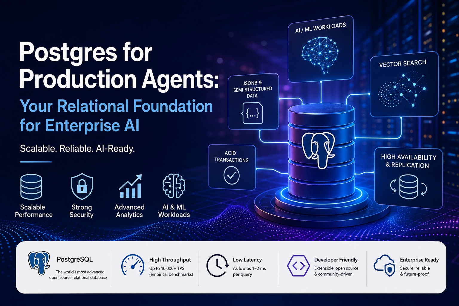
Most teams building AI agents reach for a vector database as their first infrastructure decision. Gwen Shapira, co-founder and CPO of Nile, argues that is often the wrong first move: Postgres, a database most teams already run, already does most of what an agent needs, if you know which parts of it to use. This article walks through her InfoQ talk on Postgres for production AI agents in depth: what an agent actually needs from a data layer, how JSONB, pgvector, and MVCC each cover a different part of that need, and where the real performance tradeoffs sit.

The pattern Shapira is reacting to is a familiar one in infrastructure decisions generally: a team ships a prototype where semantic search over a handful of documents works well enough, and the architecture that prototype was built on, usually a standalone vector database chosen because it was the fastest way to get embeddings into a demo, gets carried forward into production without anyone re-examining whether the rest of what a production agent needs (transactional writes, relational joins, access control, backup) was ever part of that evaluation. The talk's argument is not that vector search is unimportant, pgvector gets a full third of the talk's structure, it is that vector search decided in isolation, before the rest of an agent's data requirements are on the table, tends to under-weight everything else an agent will eventually need from wherever its data lives.

Why Relational-First, Not Vector-First

The instinct to reach for a dedicated vector database comes from treating semantic search as the whole problem. In Shapira's framing, semantic search is one input among several an agent needs to act reliably. Before an LLM touches a query, there is usually a deterministic layer of facts that a relational database already answers precisely: which tickets are open, which customers are affected, what the priority distribution looks like. Her example is an AI-assisted Jira agent: instead of asking an LLM to reason from scratch about a support incident, the system first runs SQL to gather issue details, the list of affected customers, project priorities, and comparative metrics such as ticket-age percentiles and the count of P0 (highest severity) tickets. Only once that deterministic context exists does the LLM get involved, to summarize, explain, or decide on an action.

This ordering matters for a reason that has nothing to do with database choice and everything to do with reliability: a SQL aggregate is either right or it throws an error. An LLM asked to estimate the same aggregate from raw context is neither. Feeding the LLM a deterministic answer up front removes an entire class of failure before generation even starts.

It is worth walking through what "gather issue details, affected customers, priorities, and comparative metrics" actually looks like as SQL, because the shape of that query is the shape of the reliability guarantee. A ticket-age percentile and a P0 count are not exotic operations, they are the kind of aggregate window functions and common table expressions (CTEs) were built for:

-- Deterministic context for the Jira agent, computed before any LLM call
WITH ticket_ages AS (
    SELECT
        id,
        priority,
        customer_id,
        EXTRACT(EPOCH FROM (now() - created_at)) / 3600 AS age_hours
    FROM issues
    WHERE status != 'closed'
),
percentiles AS (
    SELECT
        percentile_cont(0.5) WITHIN GROUP (ORDER BY age_hours) AS p50_age_hours,
        percentile_cont(0.95) WITHIN GROUP (ORDER BY age_hours) AS p95_age_hours,
        count(*) FILTER (WHERE priority = 'P0') AS p0_count,
        count(DISTINCT customer_id) FILTER (WHERE priority = 'P0') AS p0_affected_customers
    FROM ticket_ages
)
SELECT * FROM percentiles;

Every value that query returns is auditable: re-run it and you get the same answer, because it is arithmetic over rows that exist, not a language model's best guess at what the arithmetic probably looks like. This is the property Shapira is pointing at when she says a SQL aggregate is either right or it throws an error. There is no third outcome where it is plausible-sounding but wrong, which is exactly the failure mode an LLM asked to eyeball the same numbers from a wall of ticket text is exposed to.

"You cannot ask an agent to do something that you have absolutely no idea how it would work if you did it yourself." - Gwen Shapira

This principle also reframes what "agentic" means at the database layer. Rather than a developer pre-selecting which queries an agent is allowed to run, the agent is handed a set of database tools and decides, at run time, what to query. That only works if the person designing those tools can already picture, step by step, how they would answer the question manually with SQL. If the human designer cannot trace that path, an agent cannot be expected to either. This is why the InfoQ talk spends as much time on SQL fundamentals (window functions, CTEs, joins) as it does on anything AI-specific: the agent's reliability ceiling is the same as a competent engineer's ceiling with the same tools.

Put concretely, a "tool" exposed to an agent is rarely a single hardcoded query, it is closer to a parameterized template the agent fills in: which project, which time window, which priority band. The design discipline this demands is the same discipline a human API designer applies when deciding which parameters a REST endpoint accepts. If a tool's SQL template joins issues to customers to projects and aggregates by priority, the person who wrote that template needs to already understand what each join does to row cardinality, and where a missing index would turn a 50ms tool call into a 30-second one that times out mid-agent-turn. None of that understanding is optional just because an LLM is the thing calling the tool instead of a frontend button.

The Three Jobs a Single Postgres Instance Does for an Agent

Shapira's case for Postgres rests on it covering three distinct jobs with one engine, rather than stitching together three separate systems.

Job 1: Semi-Structured Context, with JSONB

Agent context is rarely a clean relational row. It is often a payload with an unpredictable shape: a webhook body, a log line, a partially-structured API response. Postgres's JSONB type stores this kind of payload as a binary, indexable document rather than a plain text blob. Unlike storing JSON as text, JSONB supports indexing on nested keys and efficient containment queries (does this document have this key, does this array contain this value), so a query can filter a table of semi-structured agent context nearly as fast as a query against fully normalized columns. This matters at the tool-design layer described above: an agent tool that queries "all support tickets where the payload contains a specific customer tag" needs that query to come back in milliseconds, not scan every row's raw text.

The mechanism behind that speed is a GIN (Generalized Inverted Index) built over the JSONB column. A GIN index decomposes each document into its keys and values at insert time, so a containment query does not need to parse and walk every document on every read, it looks up the relevant keys directly in the index structure, the same way a book index lets you jump to a page instead of reading the whole book. Postgres exposes this through a small set of operators purpose-built for JSONB: @> for "does the left document contain the right one," ? for "does this top-level key exist," and ?& / ?| for "does this document contain all of / any of these keys."

-- Semi-structured webhook payloads with a GIN index for fast containment queries
CREATE TABLE agent_events (
    id SERIAL PRIMARY KEY,
    payload JSONB NOT NULL,
    received_at TIMESTAMPTZ NOT NULL DEFAULT now()
);

CREATE INDEX ON agent_events USING gin (payload jsonb_path_ops);

-- Fast: does this payload contain this specific customer tag?
SELECT id, payload
FROM agent_events
WHERE payload @> '{"customer_tag": "acct-4471"}';

-- Fast: does this payload have a "priority" key at all, regardless of value?
SELECT id, payload
FROM agent_events
WHERE payload ? 'priority';

The choice of jsonb_path_ops over the default GIN operator class is itself a small but real tradeoff worth naming: jsonb_path_ops builds a smaller, faster index that only supports the @> containment operator, while the default operator class supports the full set (@>, ?, ?&, ?|) at the cost of a larger index. An agent tool that only ever needs containment lookups gets a faster, more compact index by being explicit about that at index-creation time, rather than defaulting to the option that supports every possible query shape "just in case."

It is also worth being precise about where JSONB stops being the right tool. Shapira's framing is that JSONB covers the unpredictable part of an agent's context, not that it should replace normalized columns wholesale. A column you already know the shape of, and that you filter or join on constantly, belongs in a real column with a real type and a real B-tree index, because that is a strictly faster and more constrained path than pulling it out of a JSONB blob on every query. JSONB is the escape hatch for the payload that genuinely varies row to row, not a substitute for schema design.

There is also a middle ground worth naming, between a full column and an unindexed blob: an expression index on a specific nested key inside a JSONB document. If an agent tool repeatedly filters or sorts on one particular field buried inside an otherwise-variable payload, say every webhook payload happens to carry a severity field even though the rest of the document's shape is unpredictable, Postgres can index that one path directly, without requiring the whole document to be flattened into columns:

-- Index one predictable field inside an otherwise variable JSONB document
CREATE INDEX ON agent_events ((payload->>'severity'));

SELECT id, payload
FROM agent_events
WHERE payload->>'severity' = 'critical';

This is the practical middle ground between "everything is a normalized column" and "everything is opaque JSON": the fields that are stable enough to be relied on get their own index even while they stay physically inside the JSONB document, and the fields that genuinely vary stay unindexed until a query pattern proves they need it.

The same containment logic extends naturally to arrays nested inside a document, which matters because agent payloads frequently carry list-valued fields, a webhook's list of affected resource IDs, a log line's list of tags. The @> operator that checks whether one document contains another works identically when the contained value is inside a JSONB array, so "does this event's tag list include this specific tag" is the same containment query shape as "does this event have this specific top-level field," which keeps the mental model for querying JSONB consistent regardless of whether the field in question is a scalar or a list:

-- Containment works the same way against a value nested inside a JSONB array
SELECT id, payload
FROM agent_events
WHERE payload @> '{"tags": ["rate_limit_exceeded"]}';

This consistency is part of why JSONB, rather than a bespoke document format, is the natural fit for agent context specifically: an agent tool that queries "events tagged X" and a tool that queries "events with field Y set" are the same kind of query against the same index, which means an agent generating its own filter conditions at run time only needs to reason about one query pattern, not a different syntax for scalars versus arrays versus nested objects.

Job 2: Semantic Context, with pgvector

The second job is similarity search over embeddings, and this is where the pgvector extension comes in. pgvector adds a vector column type and, critically, an approximate nearest-neighbor index called HNSW (Hierarchical Navigable Small World). HNSW builds a multi-layer graph over the embedding space: a sparse top layer for coarse navigation and progressively denser lower layers, so a search starts far from the answer and narrows in a small number of hops rather than comparing the query to every stored vector. In the talk, HNSW is described as outperforming the older IVFFLAT index, reaching 90%+ recall (the fraction of true nearest neighbors actually returned) at competitive query speeds, with the caveat that its top layer needs to fit in memory to keep that speed advantage.

Concretely, an HNSW graph is built from two structural parameters set at index-creation time: m, the maximum number of graph connections each node keeps to its neighbors, and ef_construction, how many candidate neighbors the index considers while building those connections. A higher m makes the graph denser and more accurate to traverse, at the cost of more memory and slower index builds; a higher ef_construction makes the build itself more thorough, again trading build time for eventual search quality. Neither of these is a knob you tune per-query, they are baked into the index once and reflect a deliberate choice about where on the recall/speed/memory curve this particular table needs to sit.

Once the index exists, there is a second, query-time parameter: ef_search, how many candidates HNSW explores while answering a specific query. This is the one an application actually tunes live, because it is a request-level tradeoff rather than a structural one: a higher ef_search costs more latency per query in exchange for higher recall, and it can be raised for a query that matters (a compliance search that must not miss a match) and lowered for a query where approximate is fine (a "similar articles" widget).

-- Build-time parameters: denser graph, more thorough construction
CREATE INDEX ON support_tickets
USING hnsw (embedding vector_cosine_ops)
WITH (m = 16, ef_construction = 64);

-- Query-time parameter: raise recall for this specific query at the cost of latency
SET hnsw.ef_search = 100;

SELECT id, payload
FROM support_tickets
ORDER BY embedding <=> '[...]'::vector
LIMIT 20;

pgvector also exposes three distinct distance operators, and picking the wrong one silently degrades result quality without ever raising an error: <-> for Euclidean (L2) distance, <=> for cosine distance, and <#> for negative inner product. Which one is correct depends entirely on how the embedding model that produced the vectors was trained, most modern text embedding models (the kind used for RAG-style semantic search) are trained against cosine similarity, which is why <=> is the operator that shows up by default in most pgvector examples, including the ones in this article. Using L2 distance against vectors trained for cosine similarity will still return an ordering, it just will not be the ordering the embedding model actually intended.

A second lever on this same job is vector quantization: reducing the precision of each dimension in the embedding from a 32-bit float down to 8 or 16 bits. Shapira cites a 4x improvement from this change, consistently across four different resources: query speed, memory footprint, disk footprint, and network transfer, because all four scale directly with how many bytes each vector occupies. The tradeoff is recall: a coarser representation of each vector loses some precision, so the quantization level has to be tuned against how much recall loss is acceptable for the use case.

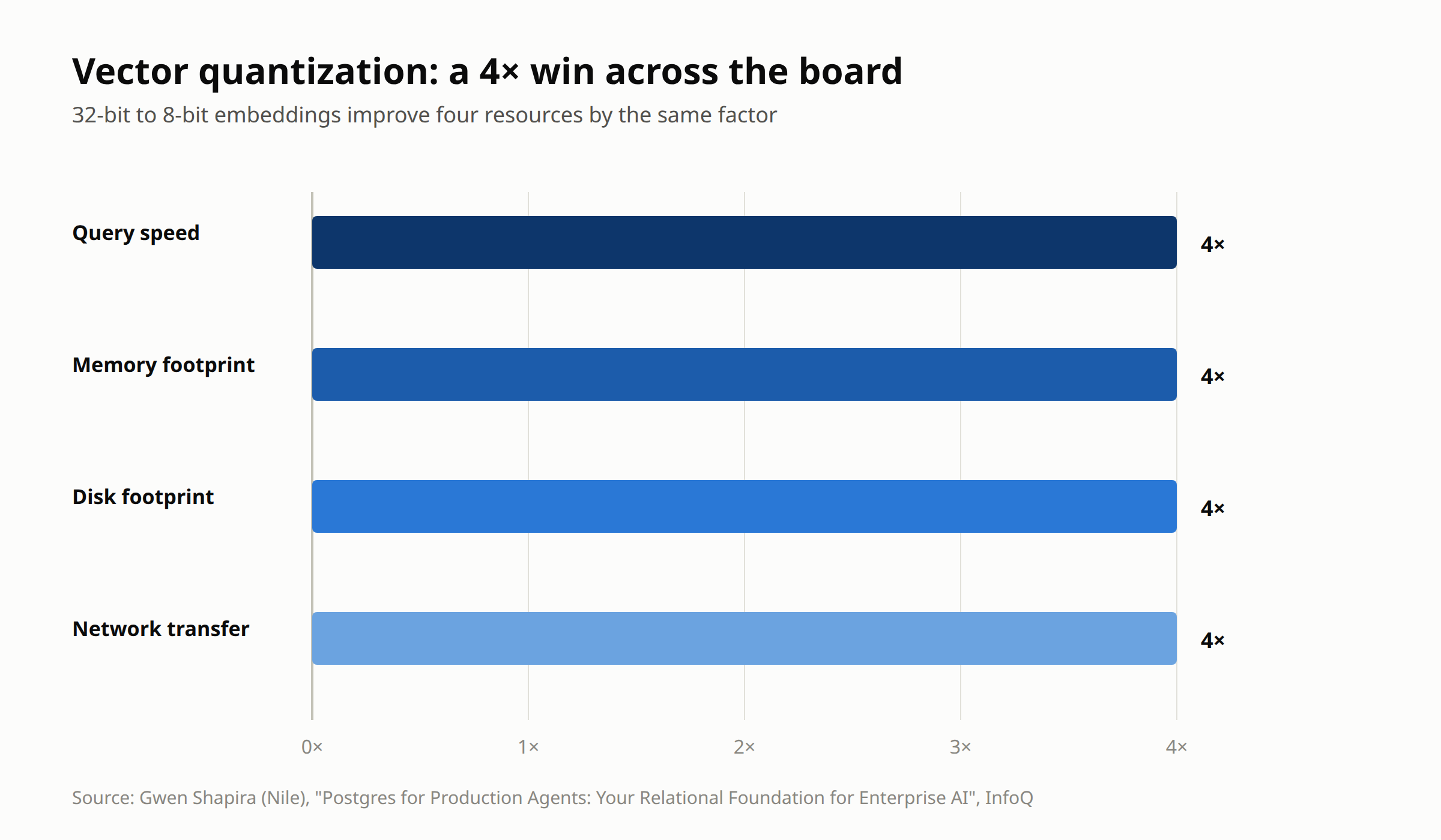
The arithmetic behind that 4x figure is straightforward once you write it out: a 32-bit float embedding at 1,536 dimensions (a common dimensionality for widely-used text embedding models) occupies 1,536 × 4 bytes = 6,144 bytes per vector before any index overhead. Halving that precision to 16 bits per dimension halves the footprint to 3,072 bytes; going further to 8 bits per dimension quarters the original footprint to 1,536 bytes. Every one of query speed, memory, disk, and network transfer is, at its core, a function of how many bytes have to move through the system, which is exactly why a single change to per-dimension precision moves all four proportionally rather than trading one off against another.

Embedding dimensionality itself varies widely by model, from 256 dimensions on the compact end up to 4,000 or more on the high-capacity end. The practical implication Shapira draws out is a scale threshold, not a hard cliff: once a table holds somewhere in the range of 3,000 to 10,000 embeddings, brute-force nearest-neighbor search (comparing the query against every row) starts visibly degrading, which is the point at which an approximate index like HNSW stops being an optimization and starts being a requirement.

-- Enable pgvector and store a 1536-dimension embedding column
CREATE EXTENSION IF NOT EXISTS vector;

CREATE TABLE support_tickets (
    id SERIAL PRIMARY KEY,
    payload JSONB NOT NULL,
    embedding vector(1536),
    created_at TIMESTAMPTZ NOT NULL DEFAULT now()
);

-- HNSW index for approximate nearest-neighbor search
CREATE INDEX ON support_tickets
USING hnsw (embedding vector_cosine_ops);

-- Nearest tickets to a query embedding
SELECT id, payload
FROM support_tickets
ORDER BY embedding <=> '[...]'::vector
LIMIT 20;

One operational detail worth calling out: HNSW's default search behavior looks at roughly 200 nearest candidates before any downstream filtering is applied, then iterates further if too few candidates survive that filter. Any query that combines a vector search with a strict WHERE clause, for example "similar tickets, but only from this customer," needs to account for this: a filter that is too selective on top of an approximate search can starve the query of candidates and silently return fewer or lower-quality results than expected. This is exactly the kind of failure mode that is invisible in a demo with a small dataset and only shows up under real data volume.

The practical mitigation follows directly from understanding the mechanism: if a filtered vector query is returning suspiciously few or low-quality results, the first thing to check is whether the candidate pool HNSW is drawing from before filtering is large enough to survive the filter. Raising ef_search widens that candidate pool at the cost of latency, which is a reasonable trade for a query where the filter is known to be highly selective, a customer with only a handful of tickets is exactly the case where the default 200-candidate pool can be exhausted by the filter before 20 good results survive it.

It is worth being precise about why HNSW's traversal is fast in the first place, because the speedup is not free, it is a direct consequence of the graph structure trading completeness for hops. A brute-force search against N stored vectors has to compute a distance for every one of them, cost that grows linearly with table size. HNSW instead enters the graph at its sparse top layer, jumps toward the query vector across a handful of long-range connections, then drops down a layer and repeats with progressively shorter, denser connections, until the bottom layer's local neighborhood is reached. Each layer narrows the search space by roughly an order of magnitude, which is why the number of distance computations an HNSW query performs grows logarithmically with table size rather than linearly. The "approximate" in approximate nearest neighbor comes from exactly this: a query that takes a slightly different path through the graph, because ef_search was set lower, or because the graph itself was built with a lower m, can settle on a local neighborhood that is very good but not provably the single best one, which is the recall tradeoff the whole index is built around.

Job 3: Safe Concurrent Access, with Transactions and MVCC

The third job is the one least associated with AI workloads: transactional concurrency. Multiple agents, or multiple instances of the same agent, often need to work off a shared queue of tasks without stepping on each other, an agent picking up a task that another agent already claimed is a correctness bug, not a performance detail. Postgres's MVCC (Multi-Version Concurrency Control) model, combined with row-level locking, gives a direct mechanism for this: an agent can SELECT ... FOR UPDATE SKIP LOCKED to atomically claim the next unclaimed row from a table acting as a work queue, without a separate message broker.

It helps to be explicit about what each piece of that clause is doing, because the three components solve three separate problems. SELECT ... FOR UPDATE alone acquires a row lock on whatever it selects, which stops a second transaction from also acquiring a lock on that same row until the first transaction commits or rolls back, that is what makes the claim atomic. Without SKIP LOCKED, though, a second agent's SELECT ... FOR UPDATE against an already-locked row does not fail, it blocks, waiting for the first transaction to release the lock. For a task queue with several concurrent agent workers, that blocking behavior is exactly wrong: every worker after the first would queue up waiting on whichever row the previous worker happened to grab, turning a queue meant to parallelize work into a line of workers taking turns. SKIP LOCKED changes that blocking wait into a skip, a worker that tries to lock an already-locked row simply moves on to the next candidate row instead of waiting, which is what lets multiple agents pull from the same queue in parallel without contention.

It is worth contrasting this directly with what a queue built without SKIP LOCKED actually does under load, since the failure mode is easy to underestimate until it is described concretely. Picture five agent workers all polling the same agent_tasks table with a plain SELECT ... FOR UPDATE and no SKIP LOCKED. The first worker to run locks the top row and starts processing it. The other four workers' SELECT statements, ordered by created_at the same way, all land on that same top row, find it locked, and block, waiting. None of them advance to the second row, because none of them have been told they are allowed to skip a locked row and look further down the list, they are simply waiting for the specific row they asked for. The five-worker queue behaves, for as long as that first task takes to process, exactly like a one-worker queue, with four workers doing nothing but waiting on a lock. SKIP LOCKED is the one keyword that turns that into genuine parallelism, by telling each worker's query to treat a locked row as absent rather than as something to wait for.

MVCC is the layer underneath that makes any of this safe without heavier locking. Rather than locking an entire table or blocking readers while a row is being updated, Postgres keeps multiple versions of a row simultaneously, each transaction sees a consistent snapshot of the data as of when it started, regardless of what other concurrent transactions are doing to the same rows. This is why a long-running agent transaction reading task history does not block a second agent claiming a new task, and why a task claim does not require locking anything beyond the specific row being claimed.

It is worth being explicit about the scope of what MVCC's default snapshot isolation guarantees, because it is a guarantee about read consistency within a transaction, not a substitute for the row-level locking the queue pattern relies on. Under Postgres's default read-committed isolation, each individual statement within a transaction sees a fresh snapshot as of when that statement started, which is enough to prevent one agent from reading a half-committed write from another, but it does not by itself prevent two agents from both deciding to claim the same row if they evaluate their WHERE clause at the same instant. That race is closed specifically by the row lock FOR UPDATE takes out, not by isolation level alone, which is exactly why the queue-claiming pattern combines a row lock with SKIP LOCKED rather than relying on transaction isolation to do that job on its own.

-- Claim the next unclaimed task, skipping rows another agent already locked
BEGIN;

SELECT id, task_payload
FROM agent_tasks
WHERE status = 'pending'
ORDER BY created_at
FOR UPDATE SKIP LOCKED
LIMIT 1;

UPDATE agent_tasks SET status = 'in_progress' WHERE id = $1;

COMMIT;

A queue built this way still needs an answer for the case where an agent claims a task, updates its status to in_progress, and then crashes or times out before completing it, since the row is no longer pending, the pattern above alone would leave it stuck forever. The standard extension of this pattern adds a claimed_at timestamp alongside the status column, and widens the queue's WHERE clause to also reclaim rows that have been in_progress for longer than some lease window, treating a stale claim the same as no claim at all:

-- Reclaim tasks whose lease has expired, alongside genuinely unclaimed ones
SELECT id, task_payload
FROM agent_tasks
WHERE status = 'pending'
   OR (status = 'in_progress' AND claimed_at < now() - interval '5 minutes')
ORDER BY created_at
FOR UPDATE SKIP LOCKED
LIMIT 1;

This pattern is not a novel trick, it is a standard use of row-level locks that predates AI agents by decades, but it is precisely the kind of primitive that a bespoke vector-only datastore does not give you. Reaching for Postgres means this concurrency problem is already solved by the engine, rather than requiring a second system just to coordinate which agent does what.

There is one operational cost worth naming honestly rather than glossing over: a task queue table under MVCC accumulates dead row versions every time a row is updated (claimed, then completed, then perhaps archived), because MVCC keeps old versions around until they are no longer visible to any in-flight transaction. Postgres's autovacuum process reclaims that space in the background, but a queue table with a high churn rate, many agents claiming and completing many short tasks, is exactly the kind of table where autovacuum tuning (more aggressive vacuum thresholds, or a more frequent schedule specifically for that table) is worth doing deliberately rather than leaving on defaults. This is not a reason to avoid the pattern, it is a reason to monitor table bloat on high-throughput queue tables the same way you would monitor any other production hot path.

Validate Retrieval Before Trusting the LLM With It

A recurring warning in the talk is to check similarity search results before they ever reach the language model. Shapira's phrasing is blunt: "LLMs are so convincing, it's so easy to trick yourself." A retrieval bug, an HNSW query that silently returned zero relevant results after an overly strict filter, or a stale embedding that no longer matches its source row, does not surface as an error. It surfaces as a fluent, confident, wrong answer, because the LLM will happily generate a plausible-sounding response from whatever context it was handed, correct or not. The practical implication is to treat retrieval as a component with its own test suite: spot-check that the top-K results for a known query are the ones you expect, before wiring that retrieval path into a chain that ends in an LLM call.

Two of the specific failure modes named earlier in the talk map directly onto this validation discipline. The overly-strict-filter-plus-HNSW problem described above is one concrete instance of "a retrieval bug that does not surface as an error": if the candidate pool is starved by a filter, the query still returns a result set, it is just a smaller and lower-quality one than it should be, and nothing in the response shape flags that degradation. A test suite that only checks "did the query return something" will pass on a starved query exactly as readily as it passes on a healthy one; the check that actually catches this compares the returned set against a known-good expected set for a fixed test query, not just checks for non-emptiness.

The stale-embedding failure mode deserves its own discipline for the same reason: an embedding column is a derived value, computed once from a source row's text at some point in time, and nothing in Postgres automatically knows to recompute it when the source text changes, or when the embedding model itself is upgraded. A row updated after its embedding was generated will keep matching queries as if its old content were still current, which is invisible unless the system explicitly tracks when each embedding was generated relative to when its source row last changed:

-- Track embedding staleness explicitly rather than assuming freshness
ALTER TABLE support_tickets ADD COLUMN embedding_generated_at TIMESTAMPTZ;
ALTER TABLE support_tickets ADD COLUMN content_updated_at TIMESTAMPTZ NOT NULL DEFAULT now();

-- Find rows whose embedding predates their content, ie. stale embeddings
SELECT id
FROM support_tickets
WHERE embedding_generated_at IS NULL
   OR embedding_generated_at < content_updated_at;

None of this replaces validating the LLM's final output, it happens strictly before that, on the assumption that a wrong retrieval guarantees a wrong or misleading answer downstream no matter how good the language model is. Treating retrieval as trustworthy by default, rather than as a component that gets its own regression tests, is the gap Shapira is pointing at with the warning about how convincing LLMs are: the model's fluency actively works against noticing that the input it was given was already wrong.

A useful discipline for building the "test suite for retrieval" Shapira describes is to maintain a small, fixed set of test queries with hand-verified expected results, the same way a human-facing search feature would maintain a golden set of query/expected-result pairs for regression testing. Every time the embedding model, the HNSW parameters, or the underlying data changes, that fixed set gets re-run and compared against its expected results before the change ships. This is a deliberately low-tech answer to a problem that is otherwise easy to over-engineer: it does not require a separate evaluation framework, it requires picking a handful of queries an engineer already knows the right answer to, and refusing to ship a retrieval change that breaks them.

Why Postgres Specifically, Not Just "a Relational Database"

The case Shapira makes is not for relational databases in the abstract, it is for Postgres's specific combination of extensibility and multi-modal data support inside a single engine. JSON documents, geospatial data through the PostGIS extension, vector embeddings through pgvector, and traditional relational rows all coexist in the same database, under the same transaction guarantees, queried with the same SQL dialect. Full-text search indexes add a fourth modality, plain keyword and phrase search over document content, again in the same engine.

What "under the same transaction guarantees" buys in practice is worth spelling out with a concrete agent scenario, because it is easy to read past as a platitude. Suppose an agent needs to update a support ticket's status, append a new field to its JSONB payload, and regenerate its embedding to reflect the new content, all as a result of one action. In a single Postgres database, that is one transaction: all three writes commit together or none of them do, so a crash mid-update can never leave the row with a new status, a stale payload, and a mismatched embedding. Split across three separate systems, a relational store, a document store, and a vector database, there is no single transaction boundary spanning all three, which means the application itself has to handle the case where the status update succeeds but the embedding regeneration fails, typically with retry logic, reconciliation jobs, or an eventual-consistency window during which the row's ticket status and its embedding genuinely disagree.

The full-text search dimension is worth a concrete look too, since it solves a different problem than pgvector does even though both are described as "search." Postgres's tsvector/tsquery machinery indexes exact lexical matches, stemmed and ranked, which is the right tool for "find tickets mentioning this exact error code" in a way that semantic embedding search is not, an embedding model will happily return semantically similar tickets that never actually contain the literal string you searched for. tsvector also supports ranking a result set by relevance through ts_rank, which weights matches by how often and how prominently the search terms appear, giving an agent tool a second, independent relevance signal beyond vector distance that it can use to re-order or cross-check semantic results. Having both in the same engine means an agent tool can combine them in one query rather than merging results from two separate systems after the fact:

-- Combine exact lexical match (tsvector) with semantic similarity (pgvector)
-- in a single query, against a single consistent snapshot of the data
SELECT id, payload
FROM support_tickets
WHERE to_tsvector('english', payload->>'description') @@ to_tsquery('timeout & connection')
ORDER BY embedding <=> '[...]'::vector
LIMIT 20;

The alternative architecture, a separate document store, a separate vector database, a separate search index, and Postgres for the "actual" relational data, works, but it means every agent query that needs more than one of these modalities has to fan out across systems and reconcile consistency between them by hand.

PostGIS is worth a similarly concrete mention, since it is the modality least associated with AI agents but still directly relevant to the same architectural point: an agent tool for, say, "find affected customer sites within a given radius of an outage" is a geospatial query, not a semantic or relational one on its own, and PostGIS extends Postgres with the geometry types and spatial indexes (GiST-based, analogous in spirit to how GIN indexes JSONB and HNSW indexes vectors) needed to answer it directly in SQL. The point Shapira is making by naming PostGIS alongside pgvector and JSONB is not that every agent needs geospatial queries, most will not, it is that Postgres's extension model keeps adding modalities without changing the engine's core guarantees, so an agent architecture that starts with JSONB and pgvector does not hit a wall the day a geospatial requirement shows up; the same database keeps covering it.

Postgres also brings three decades of production hardening to this: mature backup and point-in-time recovery tooling, a security model built on row-level access control and roles, and an extension ecosystem that lets teams add capability (pgvector, PostGIS, full-text search) without replacing the underlying engine. Row-level security in particular is worth noting for agent workloads specifically: it lets the database itself enforce which rows a given agent's connection is allowed to see or modify, as a policy attached to the table rather than as logic the application has to remember to apply on every query path. For a multi-tenant agent system, where one customer's agent must never be able to read another customer's rows, enforcing that at the database layer closes off an entire class of bug that would otherwise depend on every application code path getting the tenant filter right, every time, forever. Shapira's framing is that this maturity is underappreciated in AI infrastructure conversations that default to newer, narrower tools.

What Changes When the Caller Is an Agent, Not a Human

It is worth stepping back and naming directly what is actually new about any of this, since none of the three jobs described above, semi-structured storage, similarity search, transactional concurrency, are novel Postgres capabilities invented for AI. What changes with an agent as the caller is the shape of the risk. A human engineer running an ad hoc SQL query against a slow, unindexed table notices the slowness immediately, and either fixes the query or the index before it becomes a habit. An agent running the same query as one step inside a multi-step reasoning chain has no equivalent moment of noticing: a 30-second query is, from the agent's perspective, just a slower tool response, folded into whatever plan it is executing, and the eventual answer it produces will look exactly as confident whether that tool call took 50 milliseconds or 30 seconds. The database-design discipline does not change, but the cost of skipping it changes from "an annoyed engineer" to "a silently degraded agent that nobody notices is degraded."

The same logic applies to every failure mode covered above: a starved HNSW filter, a stale embedding, a queue row claimed twice, none of these are new problems introduced by agents, they are old problems that used to have a human in the loop to notice them, replaced by a caller that will not. This is the underlying reason Shapira's talk treats "could a human trace this by hand" as the bar for whether an agent tool is trustworthy: it is not a metaphor, it is pointing at the fact that the human-in-the-loop noticing is exactly the safety net that disappears once an agent is calling the tool instead.

How the Talk Is Organized

For readers who want to go to the original presentation, the talk itself moves through six stages: what an LLM needs as context (historical, environmental, current), relational queries and JSON construction as the RAG layer, vector embeddings and semantic search, agentic tool design, memory management through transactions, and finally the case for Postgres specifically, covering reliability, extensibility, and row-level security.

That six-stage structure is itself a small argument in miniature: it starts from what an agent needs (context, historical and current), works through the three mechanisms that supply different kinds of context (relational queries, vector search, transactional memory), and only arrives at "why Postgres" after establishing what the actual requirements are. The order matters because it is the opposite of starting from a product category, vector database, and working backward to justify it; it starts from the problem and lets the requirements point at the tool.

A Practical Checklist for a Postgres-Backed Agent

• Design tools you could operate yourself: if a human cannot trace the SQL path to an answer, an agent tool built around that query is not trustworthy either.
• Put deterministic context first: run the relational aggregate before the LLM call, do not ask the model to approximate a count or a sum.
• Use JSONB for unpredictable payloads, not as a substitute for columns you already know the shape of; index it with GIN, and pick jsonb_path_ops over the default operator class when only containment queries are needed.
• Add an HNSW index once a table approaches a few thousand embeddings, brute-force nearest neighbor stops being viable well before that; tune m and ef_construction at build time, and ef_search per query when a specific request needs higher recall.
• Match the distance operator to how the embedding model was trained, cosine distance (<=>) for most modern text embedding models, not Euclidean or inner product by default.
• Tune quantization deliberately, the 4x resource win is real, but validate recall at your chosen precision before shipping it.
• Watch for filter starvation on approximate vector search, a highly selective WHERE clause on top of HNSW's default candidate pool can silently return fewer or worse results than expected.
• Use SELECT ... FOR UPDATE SKIP LOCKED for multi-agent task queues instead of introducing a separate broker for coordination Postgres already provides, and add a claim-lease timeout so a crashed worker's task gets reclaimed.
• Monitor table bloat on high-churn queue tables, MVCC's row-versioning has a real vacuum cost under heavy update traffic.
• Track embedding staleness explicitly, a source row that changed after its embedding was generated will keep matching as if nothing changed, unless you record and check for that gap.
• Validate retrieval output independently of the LLM, a wrong but fluent answer is a silent failure, not a loud one, and it is the retrieval step, not the model, that is usually at fault.

Conclusion

The throughline of Shapira's talk is that production AI agents do not need a fundamentally different data layer, they need the same reliability discipline any production system needs, applied to the tools an agent is given. Postgres already covers the three jobs that discipline requires: semi-structured storage through JSONB, semantic search through pgvector's HNSW index, and safe concurrent access through MVCC and row-level locking. The advantage of doing all three in one engine is not a performance number, it is that consistency, backup, security, and operational tooling apply uniformly across all of it, instead of being reinvented separately for a vector store, a document store, and a queue.

None of the individual mechanisms described here, GIN indexes over JSONB, HNSW's layered graph, SKIP LOCKED row claiming, are new or specific to AI. That is precisely Shapira's point: an agent does not need novel infrastructure, it needs an engineering team willing to apply infrastructure discipline that already exists, to a new class of caller that happens to be a language model instead of a human clicking a button.

For a team evaluating this today, the practical starting point is not "should we adopt Postgres" for most readers of this article, it is already the database sitting under the application. The actual decision is narrower and more concrete: before standing up a second, dedicated vector store, first ask whether pgvector on the existing instance, with an HNSW index sized and tuned as described above, already clears the latency and recall bar the use case needs. For the range of table sizes most teams are actually operating at, tens of thousands to low millions of embeddings rather than billions, Shapira's argument is that it usually does, and the operational simplicity of one engine instead of two is a real cost saved, not a hypothetical one.

Sources

• Postgres for Production Agents: Your Relational Foundation for Enterprise AI, presented by Gwen Shapira, InfoQ