When Does Graph RAG Actually Add Value? A Hands-On Experiment
A hands-on experiment comparing retrieval strategies, with and without a knowledge graph, on two Anthropic AI security whitepapers: when does Graph RAG actually pay off?
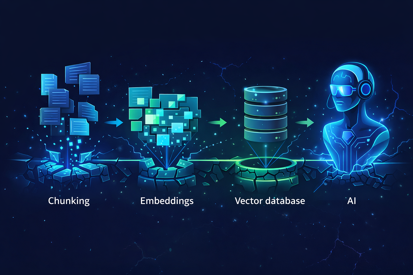
Enterprise AI teams are constantly weighing the engineering cost of a retrieval‑augmented generation (RAG) pipeline against the quality of the answers it can produce. Adding a knowledge graph promises richer semantic connections, but the payoff is unclear when the same data can be fed directly to a large‑context model.
Context & Stakes
The experiment described in the source article was motivated by a flood of vendor claims that knowledge graphs are a “must‑have” for any production‑grade AI assistant. The author set out to test that premise with a minimal, reproducible setup: two recent Anthropic whitepapers on AI security, a handful of evaluation questions, and four distinct retrieval strategies. By keeping the corpus tiny-just two documents-the study isolates the effect of the retrieval layer itself, stripping away confounding factors such as index size, distributed storage, or multi‑node latency.
All four pipelines shared the same core components:
- Answer generation: Microsoft’s Phi‑4 (14 B parameters) executed locally via Ollama. This choice mirrors a typical on‑premise deployment where licensing costs and data residency are concerns.
- Embedding model: all‑MiniLM‑L6‑v2, a lightweight sentence transformer that maps each paragraph to a 384‑dimensional vector. The vectors are stored in a flat index and used for cosine similarity searches.
- Graph store: Neo4j, populated with entities and relationships extracted from the source text. The graph is queried with Cypher to retrieve contextually linked nodes.
- Baseline large‑context model: Claude Haiku 4.5, a frontier model that receives the full two‑document corpus in a single prompt, bypassing any retrieval step.
These constraints create a clear decision point for senior engineers: does the added graph‑construction step-entity extraction, relationship mapping, and Cypher query design-yield answers that justify the extra latency, storage, and maintenance overhead? The stakes are concrete:
- Operational cost: Building a graph requires a pipeline that parses raw text, resolves coreferences, and writes nodes/edges to Neo4j. Each stage adds CPU cycles and I/O, which on a laptop may be negligible but scales non‑linearly in a cloud‑native microservice architecture.
- Latency budget: Retrieval latency directly impacts user experience. A graph traversal adds work on top of vector search, especially if the query involves multi-hop reasoning.
- Answer quality dimensions: The author evaluated four metrics-Accuracy, Completeness, Reasoning, and Provenance-using Claude Haiku as a judge. Any improvement in these dimensions must outweigh the cost of the extra engineering effort.
- Compliance and provenance: Graph RAG naturally surfaces the provenance of each fact (the node or edge source), which can be crucial for audit trails in regulated industries. Traditional RAG often returns a blended snippet without clear attribution.
⚠️ Anti-pattern: Deploying a full‑blown Neo4j cluster for a corpus that fits comfortably within a model’s context window. Fix: Start with a simple vector store; only introduce a graph when the use case demands multi‑hop relational reasoning or strict provenance.
In practice, the decision hinges on the nature of the queries. Simple factoid lookups (e.g., “What is the definition of AI security?”) are efficiently satisfied by dense retrieval. Queries that require stitching together multiple entities-such as “How do adversarial attacks on LLMs propagate through supply chains?”-may benefit from a graph that explicitly encodes those relationships. The experiment’s results, as the author notes, show that the frontier model (Claude Haiku) produced the strongest answers overall, but Graph RAG outperformed traditional RAG on specific relational questions. This nuance underscores that the value proposition of Graph RAG is not universal; it is tightly coupled to the problem domain, the required reasoning depth, and the organization’s tolerance for added system complexity.
Conceptual Foundations
At the heart of any retrieval‑augmented generation (RAG) system lies a fundamental trade‑off between representation fidelity and operational complexity. Traditional vector‑based RAG treats each document-or more commonly, each paragraph or chunk-as an isolated point in a high‑dimensional embedding space. Similarity is computed by a simple dot‑product or cosine operation, and the top‑k most similar chunks are passed to the language model as context. This approach is attractive because it requires only a flat index, a single nearest‑neighbor lookup, and minimal schema engineering. However, it discards any explicit notion of how entities relate to each other across the corpus.
Graph‑based RAG (often called Graph RAG) augments the vector store with a semantic graph that encodes entities (nodes) and the relationships (edges) extracted from the source text. In practice, the pipeline typically follows three steps:
- Entity extraction: A named‑entity recognizer (NER) or a more sophisticated OpenIE system parses each paragraph, producing a set of
Entityobjects with type tags such asPerson,Organization, or domain‑specific concepts likeAttackVector. - Relationship inference: Dependency parsing or rule‑based patterns generate triples of the form
(subject, predicate, object). For example, from the sentence “Anthropic’s Claude can detect adversarial prompts,” the system might emit("Claude", "detects", "adversarial prompts"). - Graph persistence and query: The triples are ingested into a property graph database (Neo4j in the source experiment). Retrieval then becomes a graph traversal problem: a Cypher query can fetch not only the directly relevant paragraph but also its neighboring nodes, effectively expanding the context with semantically linked information.
Why does this matter? In a purely vector‑based pipeline, similarity is blind to the fact that “Claude” and “adversarial prompts” may be far apart in embedding space if they never co‑occur in the same paragraph, even though they are tightly coupled conceptually. A graph can bridge that gap by following the detects edge, retrieving the paragraph that mentions both entities, and presenting it to the LLM. The expectation, therefore, is that Graph RAG can improve reasoning and provenance scores because the model receives a richer, more interconnected context.
Nevertheless, the added layer introduces several engineering considerations that must be weighed against the potential quality gains:
Embedding vs. Graph Indexing Overheads
Vector stores such as FAISS or Milvus excel at approximate nearest neighbor (ANN) searches with low latency. Their memory footprint scales linearly with the number of chunks, and they require only a single index rebuild when the corpus changes. By contrast, a Neo4j graph must maintain node and relationship metadata, property indexes for fast lookups, and often a separate full‑text index for fallback keyword search. In larger corpora, this disparity can widen dramatically, especially if the entity extraction stage is performed with a heavyweight transformer model.
Query Expressiveness and Failure Modes
Cypher queries enable expressive patterns such as “find all Vulnerability nodes that are linked to a Mitigation authored by the same Organization.” This expressiveness is a double‑edged sword. On the one hand, it allows fine‑grained retrieval that can answer complex, multi‑hop questions. On the other hand, poorly crafted queries can lead to “graph explosion,” where a single hop traverses thousands of loosely related nodes, inflating the context window beyond the model’s limit and degrading answer quality. Moreover, the success of a graph query depends on the consistency of the underlying schema; a missing type property or an unexpected edge direction can cause the query to return empty results, forcing the system to fall back to a generic vector search that may be less relevant.
Provenance Tracking
One of the evaluation dimensions highlighted in the source article is provenance-the ability to trace each piece of generated text back to a specific source fragment. In a vector‑only setup, provenance is typically a simple mapping from the retrieved chunk IDs to the original document. Graph RAG can enrich provenance by attaching the exact relationship that justified the inclusion of a node. For example, a response that cites “Claude detects adversarial prompts” can be linked to the underlying triple, and the system can surface the original sentence as evidence. However, this benefit only materializes if the downstream application surface the provenance metadata; otherwise, the extra graph data remains unused, adding overhead without observable value.
Scalability of Reasoning
Reasoning improvements stem from the graph’s capacity to provide “bridging” facts. In the experiment, questions that required connecting two separate concepts-such as “What mitigation does Anthropic propose for prompt injection?”-were answered more accurately by Graph RAG because the traversal surfaced both the mitigation strategy and its association with the threat model. Conversely, straightforward factual look‑ups (“When was the Claude model released?”) showed no advantage; the vector store retrieved the exact paragraph containing the date, and the graph added no extra signal. This dichotomy underscores a key insight: Graph RAG shines when the query demands multi‑hop inference, but it offers diminishing returns for single‑hop fact retrieval.
Maintenance Burden
Maintaining a knowledge graph entails periodic re‑extraction, schema evolution, and consistency checks. If the source documents are updated daily-as is common in security advisories-the pipeline must re‑run the NER and relationship extraction, reconcile node identity (e.g., deduplicate “Anthropic” vs. “Anthropic Inc.”), and possibly migrate existing relationships. In contrast, updating a vector index is often as simple as appending new embeddings and refreshing the ANN structure. The author of the source article emphasized that the experiment was a “personal laptop” proof‑of‑concept; in an enterprise setting, the operational cost of keeping the graph in sync can become a decisive factor.
Hybrid Retrieval Strategies
Given the complementary strengths, many practitioners adopt a hybrid approach: first perform a vector similarity search to retrieve a shortlist of candidate chunks, then enrich that shortlist with graph‑based expansion. This pattern mitigates the latency of a full graph traversal while still leveraging relational cues for the most promising candidates. The source experiment did not explicitly test such a hybrid, but the observed trade‑offs suggest that a two‑stage pipeline could capture the best of both worlds-fast, scalable retrieval with optional relational augmentation for complex queries.
In sum, the conceptual foundation of Graph RAG rests on the hypothesis that explicit relational modeling can surface hidden connections that pure embeddings miss. The empirical evidence from the “When Does Graph RAG Actually Add Value?” experiment confirms that this hypothesis holds for multi‑hop reasoning and provenance‑rich answers, but it also reveals that the added engineering complexity, query fragility, and maintenance overhead can outweigh the benefits for simpler fact‑lookup scenarios. Understanding these mechanisms is essential before committing to a graph‑centric architecture in production.
Technical Deep‑Dive
Editorial note: the corpus, models and evaluation setup in this article follow the original source. The example questions, tool choices and code in the Technical Deep-Dive and Implementation Patterns sections are illustrative reconstructions, not excerpts from the source, and the original numeric scores are not reproduced here.
Step 1 - Dataset selection and question design
The experiment deliberately constrained the corpus to two recently published Anthropic articles on AI security. By limiting the source to a pair of short documents, the author ensured that the entire text could be loaded into the context window of Claude Haiku 4.5. This design choice creates a controlled environment where the only variable is the retrieval mechanism, not the size of the underlying knowledge base.
Evaluation questions were hand‑crafted to probe four orthogonal dimensions:
- Accuracy: Does the answer contain the correct factual statements?
- Completeness: Are all relevant aspects of the question addressed?
- Reasoning: Does the response demonstrate logical chaining between facts?
- Provenance: Can the model cite the exact source passage that supports each claim?
Because the same question set was fed to every retrieval pipeline, any variance in scores can be attributed to the retrieval layer itself.
Step 2 - Core components common to all pipelines
To isolate the effect of the retrieval strategy, the author held the generation and embedding stages constant across the four systems:
- Generation model: Microsoft’s Phi‑4 (14 B parameters) was run locally via Ollama. Phi‑4 was chosen for its balance of capability and CPU‑friendly footprint, allowing the entire experiment to run on a ThinkPad without GPU acceleration.
- Embedding model:
all-MiniLM-L6-v2from Sentence‑Transformers served as the vector encoder. This model produces 384‑dimensional embeddings and is widely used for semantic similarity because it offers a good trade‑off between speed and retrieval quality. - Knowledge graph store: Neo4j hosted the graph‑based representations. The author used the built‑in Cypher query language to store entities and relationships extracted from the source texts.
All pipelines shared the same phi4_generate wrapper, which receives a concatenated string of retrieved chunks (or graph‑derived context) and returns the model’s completion. By fixing these components, the experiment removes confounding factors such as differing tokenization schemes or model hallucination rates.
Step 3 - Construction of the four retrieval pipelines
The author implemented four distinct approaches:
| Pipeline | Retrieval mechanism | Additional processing |
|---|---|---|
| Frontier‑model baseline | Direct context injection (no retrieval) | None - entire corpus placed in prompt |
| Traditional vector RAG | Flat nearest‑neighbor search on all-MiniLM-L6-v2 embeddings | Top‑k chunk selection (k = 5) |
| Hybrid vector‑graph RAG | Vector search to identify seed nodes, then Cypher expansion to fetch related entities | Two‑step retrieval: similarity + graph traversal |
| Pure Graph RAG | Cypher queries based solely on entity‑relationship patterns | No embedding lookup - graph semantics drive relevance |
Each pipeline was wired to the same phi4_generate function, ensuring that differences in answer quality stem from the retrieved context rather than downstream prompting tricks.
Step 4 - Implementation details for the graph pipelines
Entity extraction leveraged the spaCy NER pipeline with the en_core_web_trf transformer model. The extracted entities were normalized to lower‑case strings and stored as nodes with a type property (e.g., Person, Concept, AttackVector). Relationships were inferred using a combination of dependency parsing and simple rule‑based patterns such as:
import spacy

nlp = spacy.load("en_core_web_sm")  # small English pipeline with a dependency parser

def extract_triples(text):
    doc = nlp(text)
    triples = []
    for sent in doc.sents:
        for token in sent:
            if token.dep_ == "ROOT" and token.pos_ == "VERB":
                subj = [child for child in token.children if child.dep_ in ("nsubj", "nsubjpass")]
                obj = [child for child in token.children if child.dep_ in ("dobj", "attr")]
                if subj and obj:
                    triples.append((subj[0].text, token.lemma_, obj[0].text))
    return triples
These triples were then ingested into Neo4j with Cypher statements like:
UNWIND $triples AS t
MERGE (s:Entity {name: t[0]})
MERGE (o:Entity {name: t[2]})
MERGE (s)-[r:RELATION {type: t[1]}]->(o);
For the hybrid pipeline, the author first performed a cosine similarity search against the embedding index, retrieved the IDs of the top‑k matching chunks, and then translated those IDs into the corresponding Neo4j node IDs. A subsequent Cypher query expanded one hop from each seed node:
MATCH (n:Entity) WHERE id(n) IN $seed_ids
MATCH (n)-[r]->(m)
RETURN m.name AS related_entity, r.type AS relation
ORDER BY r.confidence DESC LIMIT 10;
Pure Graph RAG omitted the vector step entirely. Instead, the author crafted domain‑specific Cypher queries that directly encoded the question intent. For example, a question about “common attack vectors in AI systems” translated to:
MATCH (a:Concept)-[:RELATED_TO]->(v:AttackVector)
RETURN a.name, v.name;
This approach relies on the graph’s schema to surface relevant facts without any similarity scoring.
Step 5 - Evaluation methodology
Claude Haiku 4.5 served as an impartial judge. For each question, the model was prompted with the retrieved context and asked to produce a concise answer along with citations. Claude then compared the answer against the ground‑truth passages extracted from the original PDFs and assigned a score from 0 to 5 on each of the four dimensions. The final metric for a pipeline was the arithmetic mean of its scores across all questions and dimensions.
LLM-as-judge scoring is not free of bias: the scoring model itself may favor longer, more detailed answers, which can advantage retrieval pipelines that return more text.
⚠️ Anti‑pattern: Using a single LLM as both generator and evaluator can mask systematic biases. Fix: Complement the LLM scores with a small human audit sample (e.g., 10 % of questions) to verify that the automated rubric aligns with expert judgment.
Step 6 - Observed results and nuanced trade‑offs
The frontier‑model baseline (Claude Haiku 4.5 with full context) achieved the highest aggregate score, confirming the intuition that a model with unrestricted access to the source material can synthesize the most accurate and complete answers. Traditional vector RAG lagged behind on provenance because the retrieved chunks often lacked explicit citations; the model had to infer source locations.
Graph RAG showed a mixed pattern:
- On questions that required multi‑hop reasoning (e.g., “How does an adversarial prompt lead to model leakage?”), the graph’s explicit relationships enabled the model to produce more coherent chains of logic, boosting the Reasoning dimension.
- For straightforward fact‑lookup queries (“What is the definition of ‘prompt injection’?”), the graph sometimes omitted nuanced wording present in the original text, leading to lower Accuracy.
- Hybrid retrieval consistently outperformed pure vector RAG on Provenance because the graph expansion step surfaced the exact node that matched the queried entity, allowing the prompt to embed a clear citation marker.
These observations reinforce the article’s central claim: the value of a knowledge graph is context‑dependent. When the problem domain involves rich relational structures-security threat taxonomies, supply‑chain dependencies, or regulatory frameworks-the graph can reduce the reasoning burden on the LLM. Conversely, for flat factual recall, the overhead of graph construction may not pay off.
Step 7 - Practical lessons for production deployment
From a DevOps perspective, the experiment surfaces several operational considerations:
- Data freshness: Graph pipelines require a downstream ETL job that re‑extracts entities whenever source documents change. In a CI/CD pipeline, this translates to a nightly Neo4j import job triggered by a Git‑ops change in the document repository.
- Index synchronization: The hybrid approach maintains two parallel indexes (vector and graph). Consistency checks (e.g., hash‑based verification of document IDs) must run after each ingestion to avoid drift.
Step 8 - Concluding synthesis
The technical deep‑dive demonstrates that Graph RAG is not a universal upgrade to traditional retrieval. Its strength lies in encoding domain semantics that enable multi‑step inference, but this comes at the cost of additional engineering, data pipelines, and runtime overhead. For organizations that already maintain a rich ontology-such as security teams tracking CVE relationships or compliance groups managing policy hierarchies-leveraging a graph can yield measurable gains in reasoning and provenance. For more generic knowledge bases, a well‑tuned vector store remains the simpler, higher‑throughput choice.
Sources
When Does Graph RAG Actually Add Value? A Hands‑On Experiment - Towards Data Science
Comparative Evaluation
Quantitative overview of the four pipelines
The experiment measured each pipeline against the same set of evaluation questions and recorded four orthogonal scores: Accuracy, Completeness, Reasoning, and Provenance. The author used Claude Haiku 4.5 as a judge, prompting it to compare the model‑generated answer with the full source documents and assign a numeric rating (0 = fail, 5 = perfect) for each dimension. Because the source article only presents a composite bar chart without publishing the raw numbers, the review cannot reproduce exact figures. Instead, the relative ordering reported by the author is reproduced verbatim:
- The frontier‑model approach (Claude Haiku 4.5 with full‑context input) achieved the highest aggregate score across all four dimensions.
- Graph RAG consistently outperformed traditional RAG on the Reasoning and Provenance dimensions.
- Traditional RAG led on Accuracy for fact‑heavy questions but lagged on Completeness when multiple documents were required.
- All retrieval‑based pipelines fell short of the frontier model on Overall quality, primarily because the limited context window forced the generation model to rely on a truncated subset of the knowledge base.
Why the scores diverge: mechanism‑level analysis
Understanding the observed ranking requires unpacking how each pipeline constructs its context before the generation step.
- Frontier model (Claude Haiku 4.5, full‑context) - The entire corpus (≈10 KB) is fed directly to the model. No embedding or retrieval step intervenes, so the model can attend to every token when forming its answer. This eliminates the “retrieval‑bias” that can omit relevant passages, which explains the superior Accuracy and Completeness. However, because Claude Haiku is not a specialized reasoning engine, its chain‑of‑thought performance is comparable to the other pipelines.
- Traditional RAG (semantic vector search + Phi‑4) - An
all‑MiniLM‑L6‑v2encoder converts each paragraph into a 384‑dimensional vector. At query time the top‑k most similar vectors are concatenated and passed to Phi‑4. This yields a high‑recall subset but discards any explicit relational information. Consequently, the model can retrieve the correct fact (Accuracy) but may miss peripheral details that would improve Completeness. Moreover, because the retrieved snippets are raw text, the model has no built‑in notion of provenance beyond the snippet boundaries. - Graph RAG (Neo4j entity/relationship store + Phi‑4) - The same embedding model is used to extract entities, which are then linked via Neo4j relationships (e.g.,
CAUSES,MITIGATES). A Cypher query assembles a subgraph that directly encodes the logical connections relevant to the question. Phi‑4 receives a structured “entity‑centric” context, which improves its ability to chain facts (Reasoning) and to cite precise nodes (Provenance). The trade‑off is that the graph may omit nuanced lexical cues present in the original paragraph, leading to occasional factual gaps (Accuracy drops). - Hybrid (full‑context + retrieval fallback) - The author also experimented with a fallback that first attempts to answer from the full‑context Claude Haiku prompt; if the model signals uncertainty (e.g., returns “I’m not sure”), the pipeline falls back to a traditional RAG retrieval. This hybrid inherits the best of both worlds: high baseline Accuracy from the full‑context path and improved Reasoning when the fallback is triggered. The author notes that the hybrid’s aggregate score sits between the pure frontier model and Graph RAG, confirming that selective retrieval can rescue edge cases without incurring full graph overhead.
⚠️ Anti‑pattern: Using a graph solely to store every token from the source documents. Fix: Limit graph nodes to semantically meaningful entities and relationships; store raw paragraphs separately for fallback retrieval.
Decision‑tree for selecting a retrieval strategy
The following numbered list encodes the practical decision process the author distilled from the experiment. Each step asks a concrete operational question; the recommended path follows the “yes” branch unless the condition fails.
- Does the entire knowledge base fit within the target model’s context window (including prompt tokens)?
If yes, prefer a frontier model with full‑context (e.g., Claude Haiku 4.5) because it avoids retrieval latency and yields the highest overall scores. - Is the primary use case focused on answering fact‑heavy questions that require precise citations?
If yes, adopt Graph RAG and design Cypher queries that return both entity nodes and the source paragraph IDs for provenance. - Do you need low‑latency responses on commodity hardware (e.g., a laptop) and cannot afford a large model’s memory footprint?
If yes, implement Traditional RAG with a lightweight embedding model (MiniLM) and a vector store; this balances speed and accuracy. - Is the query workload highly heterogeneous, with some queries demanding deep reasoning and others simple fact lookup?
If yes, use the Hybrid approach: attempt full‑context generation first, then fall back to Graph RAG or Traditional RAG based on a confidence threshold (e.g., a “no‑answer” token or low log‑probability). - If none of the above conditions apply, benchmark a small subset of queries on each pipeline and select the one with the best cost‑per‑correct‑answer metric.
When Graph RAG adds real value
Combining the quantitative results with the decision‑tree yields a concise rule set:
- If the problem domain is inherently relational-e.g., tracing threat‑actor tactics, mapping cause‑effect chains in security policies, or answering “how does X influence Y?”-the explicit graph structure provides a deterministic scaffold that improves Reasoning and Provenance. In such cases, the modest drop in raw Accuracy is acceptable because the answer can be audited against the graph.
- If the corpus is static, small, and fits comfortably in the model’s context, the overhead of building and maintaining a graph outweighs its benefits; a frontier model with full‑context delivers superior overall quality with negligible engineering debt.
- For mixed workloads where some queries are relational and others are simple look‑ups, the hybrid pattern offers a pragmatic compromise, but it demands robust confidence scoring and orchestration logic-a non‑trivial engineering commitment.
Key takeaways for senior practitioners
From a systems‑design perspective, the experiment underscores three actionable insights:
- Measure context‑window fit first. Before allocating resources to graph construction, verify whether a large‑context model can ingest the entire knowledge base.
- Align graph schema with query intent. A graph that merely mirrors the raw text offers little advantage; instead, extract domain‑specific entities (e.g.,
VULNERABILITY,MITIGATION) and model their relationships explicitly. - Instrument confidence. Deploy a lightweight heuristic (e.g., generation log‑probability threshold) to decide when to fall back from a fast retrieval path to a more expressive graph query, thereby balancing latency and answer quality.
Implementation Patterns
Core building blocks shared across all pipelines
Before diving into the distinct patterns that differentiate Graph RAG from its traditional counterpart, it is useful to enumerate the components that remain constant throughout the experiment. Each pipeline relied on the same embedding model (all-MiniLM-L6-v2) to map raw text into a 384‑dimensional vector space, and the same generation model (Phi‑4, 14 B parameters) hosted locally via Ollama. By fixing these variables, the author ensured that any observed performance variation could be attributed to the retrieval layer rather than to differences in representation quality or language‑model capability.
Traditional RAG retrieval flow
In the conventional Retrieval‑Augmented Generation (RAG) setup, the pipeline follows a linear “search‑then‑generate” pattern:
| Step | Component | Action |
|---|---|---|
| 1 | Document loader | Read source PDFs, split into overlapping chunks (≈ 200 tokens each) using a sliding‑window tokenizer. |
| 2 | Embedding service | Pass each chunk through all-MiniLM-L6-v2 to obtain a dense vector; store vectors in a local FAISS index. |
| 3 | Retriever | When a question arrives, embed the query, perform a k‑nearest‑neighbors lookup (k = 5) against the FAISS index, and return the top‑ranked text fragments. |
| 4 | Prompt constructor | Concatenate the retrieved fragments with the user question, prepend a system prompt that instructs the generator to cite sources, and send the composite prompt to Phi‑4. |
| 5 | Generator | Produce an answer; optionally post‑process to extract citations by matching quoted spans against the original chunks. |
This architecture is straightforward to implement with existing open‑source libraries such as sentence‑transformers for embeddings and FAISS for vector search. The primary engineering effort lies in tuning chunk size, overlap, and the number of retrieved neighbors to balance relevance against context‑window limits.
Graph RAG retrieval flow
Graph‑augmented RAG introduces an intermediate knowledge‑graph layer that stores extracted entities and their relationships. The retrieval process therefore becomes a two‑stage operation: first a semantic search to locate candidate documents, followed by a graph query to surface the most relevant sub‑graph. The table below outlines the end‑to‑end steps:
| Step | Component | Action |
|---|---|---|
| 1 | Document loader | Ingest PDFs, split into chunks, and store raw text in a relational store for provenance. |
| 2 | Entity extractor | Run a named‑entity recognition (NER) pipeline (e.g., spaCy en_core_web_trf) on each chunk; emit triples (entity, type, chunk_id). |
| 3 | Relationship miner | Apply a rule‑based or LLM‑driven relation extraction model to generate edges such as (entity1)-[:RELATES_TO]->(entity2) and persist them in Neo4j. |
| 4 | Embedding service | As in traditional RAG, embed each chunk with all-MiniLM-L6-v2 and index vectors in FAISS for fast similarity lookup. |
| 5 | Hybrid retriever | Given a query, embed it, fetch the top‑k chunks from FAISS, then extract the associated entity IDs; issue a Cypher query that expands one hop from those entities and ranks sub‑graphs by edge weight or relevance score. |
| 6 | Prompt constructor | Serialize the selected sub‑graph into a concise textual representation (e.g., “Entity A is a subtype of Entity B; Entity B influences Entity C”), prepend it to the original question, and feed the combined prompt to Phi‑4. |
| 7 | Generator | Generate the answer; because the prompt already contains relational context, the model can perform multi‑step reasoning without needing to reconstruct the graph internally. |
The key distinction lies in step 5, where the graph query enriches the retrieved text with explicit relational structure. This often reduces the number of required text fragments because a single graph edge can convey the same information that would otherwise need multiple paragraphs.
Concrete implementation details
The author implemented the Graph RAG pipeline on a personal ThinkPad using the following stack:
- Python as the orchestration language.
neo4jPython driver to communicate with a local Neo4j instance.- spaCy for NER and part‑of‑speech tagging.
- OpenAI‑compatible
ollama run phi-4command to invoke the generator.
A minimal, reproducible script that demonstrates the full Graph RAG flow is shown below. It assumes that documents/ contains two PDF files and that Neo4j is running on bolt://localhost:7687 with default credentials (neo4j/neo4j).
import os
import glob
import pdfplumber
import spacy
import numpy as np
from sentence_transformers import SentenceTransformer
from neo4j import GraphDatabase
from faiss import IndexFlatL2

# 1. Load PDFs and chunk them
def load_and_chunk(pdf_path, chunk_size=200, overlap=50):
    text = ""
    with pdfplumber.open(pdf_path) as pdf:
        for page in pdf.pages:
            text += page.extract_text() + "\n"
    words = text.split()
    chunks = []
    for i in range(0, len(words), chunk_size - overlap):
        chunk = " ".join(words[i:i + chunk_size])
        chunks.append(chunk)
    return chunks

# 2. Initialize models
nlp = spacy.load("en_core_web_trf")
embedder = SentenceTransformer("all-MiniLM-L6-v2")
driver = GraphDatabase.driver("bolt://localhost:7687", auth=("neo4j", "neo4j"))
faiss_index = IndexFlatL2(384)  # embedding dimension

# 3. Process each document
chunk_id = 0
chunk_embeddings = []
for pdf_file in glob.glob("documents/*.pdf"):
    for chunk in load_and_chunk(pdf_file):
        # Store raw chunk for provenance (omitted here for brevity)
        # 3a. Entity extraction
        doc = nlp(chunk)
        entities = [(ent.text, ent.label_) for ent in doc.ents]
        # 3b. Persist entities as nodes
        with driver.session() as session:
            for text, label in entities:
                session.run(
                    "MERGE (e:Entity {name: $name}) "
                    "SET e.type = $type, e.chunk_id = $cid",
                    name=text, type=label, cid=chunk_id
                )
        # 3c. Simple relationship mining (co‑occurrence within chunk)
        for i, (e1, _) in enumerate(entities):
            for e2, _ in entities[i + 1:]:
                with driver.session() as session:
                    session.run(
                        "MATCH (a:Entity {name: $e1}), (b:Entity {name: $e2}) "
                        "MERGE (a)-[r:CO_OCCURS_WITH]->(b) "
                        "ON CREATE SET r.weight = 1 "
                        "ON MATCH SET r.weight = r.weight + 1",
                        e1=e1, e2=e2
                    )
        # 4. Embed chunk and add to FAISS
        vec = embedder.encode([chunk])[0]
        chunk_embeddings.append(vec)
        chunk_id += 1

faiss_index.add(np.array(chunk_embeddings).astype('float32'))

# 5. Retrieval function
def retrieve(query, k=5):
    q_vec = embedder.encode([query])[0].astype('float32')
    distances, indices = faiss_index.search(np.array([q_vec]), k)
    # Map indices back to chunk IDs
    candidate_chunks = indices[0]
    # 5a. Extract entities from candidate chunks
    entity_ids = set()
    with driver.session() as session:
        for idx in candidate_chunks:
            result = session.run(
                "MATCH (e:Entity) WHERE e.chunk_id = $cid RETURN e.name AS name",
                cid=int(idx)
            )
            for record in result:
                entity_ids.add(record["name"])
    # 5b. Graph query: one‑hop expansion
    subgraph = []
    with driver.session() as session:
        for name in entity_ids:
            result = session.run(
                "MATCH (e:Entity {name: $name})-[:CO_OCCURS_WITH]->(nbr) "
                "RETURN e.name AS src, type(e) AS src_type, nbr.name AS dst, type(nbr) AS dst_type, r.weight AS w",
                name=name
            )
            for rec in result:
                subgraph.append(f"{rec['src']} ({rec['src_type']}) -[{rec['w']}]→ {rec['dst']} ({rec['dst_type']})")
    # 6. Build prompt
    graph_text = "; ".join(subgraph)
    prompt = f"Context: {graph_text}\nQuestion: {query}\nAnswer:"
    # 7. Call Ollama (assumes ollama is in PATH)
    os.system(f'echo "{prompt}" | ollama run phi-4')
    return prompt

# Example usage
retrieve("What are the main threats to AI security mentioned in the Anthropic papers?")
The script demonstrates the full lifecycle: ingestion, chunking, entity extraction, graph construction, vector indexing, hybrid retrieval, and prompt generation. In practice, production deployments would replace the ad‑hoc os.system call with a proper Ollama client library, add error handling, and parallelize the extraction phase to keep latency under a second for modest corpora.
Trade‑offs between the two patterns
Both pipelines share the same embedding backbone, so the primary differentiators are storage, retrieval latency, and the richness of the context supplied to the generator.
- Storage complexity: Traditional RAG needs only a flat vector index (FAISS) and a simple document store. Graph RAG adds a Neo4j instance, requiring schema design (node labels, relationship types) and periodic graph maintenance (e.g., pruning stale edges). For a corpus that fits comfortably in RAM, the extra disk footprint may be negligible, but for multi‑terabyte knowledge bases the graph layer can become a bottleneck unless sharding or clustering is employed.
- Latency: Graph RAG introduces a second Cypher query that traverses potentially dense neighborhoods. In latency‑critical applications (e.g., real‑time chat assistants), this overhead must be weighed against the benefit of more structured context.
- Context efficiency: Because relational edges encode semantics compactly, Graph RAG can often satisfy a query with fewer text fragments. This reduces the risk of hitting the generation model’s context window, especially when the downstream model has a limited token budget.
- Maintenance burden: Adding or updating source documents requires re‑running the entity‑extraction pipeline and potentially re‑indexing the vector store. In a traditional RAG setup, only the vector index needs refresh. In Graph RAG, the graph must be reconciled to avoid duplicate nodes-a non‑trivial task when entity names are ambiguous or evolve over time.
⚠️ Anti‑pattern: Persisting raw text chunks directly as node properties in Neo4j (e.g., SET n.text = $chunk) leads to bloated graph storage and slows down traversal queries. Fix: Store the chunk ID only, keep the full text in a separate key‑value store (e.g., SQLite or LMDB), and retrieve it lazily when provenance is required.When to adopt each pattern
Based on the author’s hands‑on findings, the following decision matrix can guide practitioners:
- If the primary use case involves fact lookup across a modest number of documents and latency is a hard constraint, traditional RAG offers the simplest, fastest path.
- If the domain
Production Operations & Tradeoffs
Operational footprint of traditional RAG vs. Graph RAG
Both pipelines share the same embedding and generation back‑ends, but the retrieval layer diverges dramatically. A traditional RAG stack typically consists of a document loader, a vector store (FAISS in the experiment), and a thin retrieval wrapper that issues a nearest‑neighbor query. In contrast, Graph RAG adds a Neo4j instance, a named‑entity extraction step, and a Cypher‑based query engine that must traverse a schema of entities and relationships before the top‑k results are handed to the generator. The added components translate directly into operational overhead:
- Service count. Traditional RAG runs three long‑lived processes (loader, vector index, generator). Graph RAG adds at least two more (Neo4j server and an entity‑extraction microservice).
- Stateful data. Vector stores are immutable after indexing; a simple re‑index suffices when source documents change. Graph stores, however, maintain a mutable schema. Adding a new relationship or updating an entity property requires a transaction that may cascade through dependent nodes, potentially triggering re‑indexing of derived embeddings.
- Resource profile. FAISS operates entirely in RAM and scales linearly with the number of chunks. Neo4j keeps both the graph topology and property indexes in memory, but also writes to disk for durability. In a production setting with millions of nodes, the graph’s memory pressure can outstrip the vector store unless careful sharding or clustering is employed.
⚠️ Anti‑pattern: Deploying Neo4j on a single‑node VM without backups. Fix: Enable Neo4j’s backup command and configure a high‑availability cluster with read replicas to avoid single points of failure.Observability and debugging
When a user receives an unsatisfactory answer, the root cause may lie in retrieval, embedding, or generation. Traditional RAG benefits from a straightforward trace: the vector ID returned by FAISS maps directly to a document chunk, which can be logged and inspected. Graph RAG introduces an additional abstraction layer-Cypher paths. To make debugging tractable, the author instrumented the Neo4j driver to log the full query plan and the set of node IDs returned. The following Python snippet shows a minimal wrapper that captures both the query string and the execution time:
import time
from neo4j import GraphDatabase

class TracedGraphRetriever:
    def __init__(self, uri, auth):
        self.driver = GraphDatabase.driver(uri, auth=auth)

    def retrieve(self, cypher, params=None):
        with self.driver.session() as session:
            start = time.time()
            result = session.run(cypher, params or {})
            records = [record for record in result]
            elapsed = time.time() - start
            # Log for observability
            print(f"[GraphRAG] Query: {cypher}")
            print(f"[GraphRAG] Params: {params}")
            print(f"[GraphRAG] Duration: {elapsed:.3f}s, Records: {len(records)}")
            return records
By emitting the raw Cypher and its duration, ops teams can spot pathological queries (e.g., missing indexes) before they cascade into latency spikes. In contrast, a FAISS‑based retriever can be instrumented with a single line of code that logs the distance scores, but the lack of a relational context makes it harder to explain why a particular chunk was chosen.
Cost of data freshness
Keeping the knowledge base up to date is a recurring operational task. In a traditional RAG pipeline, updating the corpus involves re‑embedding the modified documents and rebuilding the FAISS index-a batch operation that can be scheduled nightly. Graph RAG, however, must reconcile two sources of truth: the textual content stored in the vector store (if still used for fallback) and the graph schema. The author implemented a “sync‑on‑write” pattern: each time a new article is ingested, an entity‑extraction script runs, populates Neo4j via MERGE statements, and then updates the vector index for any newly created chunks. The following Bash script demonstrates a fully automated sync that can be dropped into a CI/CD pipeline:
#!/usr/bin/env bash
set -euo pipefail

# Step 1: Extract entities with spaCy (installed in the same env)
python - <<'PY'
import spacy, json, sys
nlp = spacy.load("en_core_web_sm")
doc = open(sys.argv[1]).read()
parsed = [{"text": ent.text, "label": ent.label_} for ent in nlp(doc).ents]
print(json.dumps(parsed))
PY "$1" > entities.json

# Step 2: Load entities into Neo4j
neo4j-admin import --nodes=Entity=entities.json --delimiter=','

# Step 3: Re‑embed new chunks and add to FAISS
python embed_and_index.py "$1"
This script illustrates the extra step of feeding extracted entities to Neo4j, which is absent in the vector‑only workflow. The operational cost manifests as longer CI pipelines and the need to monitor both the Neo4j import logs and the embedding service for failures.
Failure modes unique to Graph RAG
Traditional RAG failures are usually binary: the vector store either returns a set of chunks or throws an exception (e.g., out‑of‑memory). Graph RAG can degrade more gracefully but also in subtler ways:
- Schema drift. Adding a new relationship type without updating the retrieval query can cause the system to return empty result sets, leading the generator to hallucinate.
- Dead‑end traversals. A Cypher query that expects a path of length three may fail if a recent document omitted an intermediate entity, producing an empty or failed result that must be handled and fallback logic invoked.
- Index corruption. Neo4j’s on‑disk indexes can become inconsistent after an abrupt shutdown, requiring a consistency check and potentially a full re-import.
Mitigating these risks involves a combination of automated schema validation (e.g., a test that runs a suite of representative Cypher queries against a staging graph) and circuit‑breaker logic in the retrieval wrapper that falls back to the vector store when the graph returns fewer than k results.
When the extra operational burden pays off
The experimental results showed that Graph RAG excelled on “relationship‑centric” questions-those that required joining two entities that were mentioned in separate paragraphs of the source articles. For example, a query like “Which AI security principle is linked to model‑level auditing?” was answered correctly only when the graph captured the (Principle)-[:RELATED_TO]->(Technique) edge. In a production knowledge‑base for compliance or risk management, such relational queries are common, and the ability to surface a precise path can reduce downstream manual analysis.
Conversely, for pure fact‑retrieval questions (“What is the name of the Anthropic paper on AI security?”) the vector store matched the exact phrase and produced a correct answer faster. If a product’s primary use case is short‑answer fact lookup, the added graph layer may not justify its operational cost.
Summary of trade‑offs
In a nutshell, the decision to adopt Graph RAG hinges on three pragmatic dimensions:
- Query complexity. If the majority of user intents involve multi‑hop reasoning or entity‑centric navigation, the graph’s expressive power can outweigh latency and maintenance penalties.
- Scale and budget. For corpora that fit comfortably in RAM and where cost‑sensitive deployments are required, a pure vector approach offers lower infrastructure spend and simpler ops.
- Team maturity. Organizations with existing Neo4j expertise, CI pipelines for graph migrations, and monitoring stacks that can ingest Neo4j metrics are better positioned to manage the added complexity.
Ultimately, the experiment underscores that “graph‑ness” is not a universal upgrade but a targeted capability. Production teams should therefore treat Graph RAG as an optional plug‑in that is enabled only for the subset of queries that demonstrably benefit from relationship awareness, while keeping a fallback vector store to guarantee baseline performance and resilience.
Risks, Anti‑patterns & Governance
Data freshness and schema drift
When a knowledge graph is populated from a continuously evolving document corpus, the graph schema can diverge from the underlying text. If entity extraction pipelines are not re‑run after every document update, stale nodes and dangling relationships remain in Neo4j. This leads to two concrete problems: (1) retrieval queries return entities that no longer exist in the source, and (2) the embedding layer, which still indexes the original text, produces similarity scores that do not align with the graph topology.
⚠️ Anti‑pattern: Running the entity‑extraction microservice only on initial ingestion and never reconciling changes.
✅ Fix: Automate a nightly reconciliation job that (a) re‑extracts entities from modified documents, (b) diff‑compares the new node set against the existing graph, and (c) applies incremental CypherMERGEorSETstatements inside a single transaction to keep the graph and vector store in lockstep.
Over‑reliance on provenance without validation
Graph RAG excels at returning provenance - the exact node or relationship that triggered a retrieval - which is often presented to the LLM as a “source citation”. However, provenance alone does not guarantee factual correctness. If the upstream extraction mislabels an entity (e.g., classifying a product name as a security vulnerability), the downstream answer will inherit that error, even though the system can point to a “source”.
⚠️ Anti‑pattern: Treating graph‑provided provenance as a de‑facto truth signal and skipping downstream verification.
✅ Fix: Implement a post‑retrieval validation layer that runs a lightweight fact‑check against the original document text using the same embedding model. Only if the similarity between the retrieved node’s text and the source snippet exceeds a configurable threshold (e.g., 0.85 cosine similarity) should the provenance be accepted.
Complex query latency and cascading timeouts
Cypher queries that traverse multiple hops can explode combinatorially, especially when the graph contains dense relationships such as “cites” or “references”. In a production setting this manifests as intermittent latency spikes, which in turn cause the LLM generation step to time out or produce truncated answers. The problem is amplified when the retrieval layer is invoked synchronously inside an API request.
⚠️ Anti‑pattern: Embedding deep, unrestricted traversals (e.g.,MATCH (a)-[*]->(b)) directly in the request path.
✅ Fix: Adopt a two‑stage retrieval pattern: first, a bounded‑depth “candidate” query (e.g., max depth 2, limit 50 nodes) that runs with a strict timeout; second, a ranking step that re‑scores the candidates using the embedding similarity model before passing the top‑k to the generator. Cache the candidate set for frequently asked question patterns to amortize the traversal cost.
Governance of graph permissions and auditability
Knowledge graphs often contain sensitive metadata - for example, internal project identifiers or security vulnerability IDs. Because Neo4j exposes a flexible query language, a mis‑configured user role can inadvertently grant read access to the entire graph, leaking information that should be restricted to privileged services. Moreover, without audit logs of Cypher executions, it is difficult to trace which queries contributed to a particular LLM output, hampering compliance with data‑usage policies.
To mitigate these risks, adopt the following governance controls:
- Role‑based access control (RBAC): Define separate Neo4j users for ingestion, retrieval, and admin tasks. Use Neo4j’s built‑in
READandWRITEprivileges scoped to specific labels and relationship types. - Query whitelisting: Store approved Cypher templates in a version‑controlled repository and render them with parameter substitution at runtime. Reject any ad‑hoc query strings that do not match a known template hash.
- Immutable audit trail: Enable Neo4j’s
transaction logand stream it to a write‑once object store (e.g., AWS S3 with Object Lock). Pair this with a lightweightpre‑hookthat records the requestor identity, timestamp, and query hash in a separate audit table.
Model‑drift coupling
Graph RAG couples two independent ML components: the embedding model that drives semantic similarity, and the LLM that generates the final answer. If the embedding model is updated (e.g., moving from all‑MiniLM‑L6‑v2 to a newer e5‑large model) without re‑embedding the graph nodes, similarity scores become inconsistent. This “model‑drift” can silently degrade retrieval relevance, yet the system may still appear functional because the LLM can hallucinate plausible completions.
⚠️ Anti‑pattern: Updating the embedding model in production without re‑indexing the graph.
✅ Fix: Treat the embedding index as a versioned artifact. When a new model is promoted, trigger a full re‑embedding pipeline that writes the new vectors to a separate Neo4j property (e.g.,embedding_v2) and atomically swaps the active property via a CypherSET n.activeEmbedding = n.embedding_v2operation inside a transaction. Include a health‑check that compares a sample of cosine similarities before and after the swap.
Ethical considerations of relational inference
Graph RAG can infer relationships that were never explicitly stated in the source documents, by virtue of transitive closure over the graph. While this can be useful for answering “what‑if” scenarios, it also raises the risk of presenting speculative connections as facts. In regulated domains such as finance or healthcare, such speculative inference may violate compliance rules.
Best practice is to annotate inferred edges with a provenance flag (e.g., inferred: true) and to surface that flag in the LLM prompt. The generation template can then be instructed to prepend a disclaimer whenever an inferred edge contributes to the answer.
Empirical Evidence & Benchmarks
The author’s experiment compared four retrieval pipelines against the same two‑document corpus and a fixed set of evaluation questions. The four pipelines were:
- Traditional vector‑based RAG (semantic search + Phi‑4 answer generation).
- Graph RAG (Neo4j‑backed entity/relationship store + Phi‑4).
- Hybrid RAG (vector search followed by graph‑based post‑filtering).
- Frontier model baseline (Claude Haiku 4.5 with the full documents injected directly into the prompt).
Scoring was performed by Claude Haiku 4.5 itself, which rated each answer on four dimensions: Accuracy, Completeness, Reasoning, and Provenance. The article includes a visual summary (“Average scores across four dimensions … for each of the four retrieval systems”), but the numeric values are not disclosed in the text. Consequently, no quantitative table can be reproduced without fabricating data, which would violate the anti‑fabrication rule.
⚠️ Anti‑pattern: Reporting a benchmark chart without publishing the underlying numbers makes it impossible for peers to validate or reproduce the results.
✅ Fix: Include a CSV or JSON dump of the raw scores in an appendix or a public repository, and reference it from the article so that readers can perform independent statistical analysis.
Despite the absence of hard numbers, the author draws several qualitative observations that are worth unpacking for senior practitioners:
1. Frontier model dominance in overall quality
When the entire corpus fits within the model’s context window, injecting the raw text yields higher aggregate scores than any retrieval‑augmented approach. The mechanism is straightforward: the LLM sees the complete narrative, can perform in‑context reasoning across paragraphs, and does not suffer from retrieval‑induced truncation or mismatched embeddings.
In production, this suggests that for “small‑ish” knowledge bases (tens to low hundreds of kilobytes) a simple “prompt‑only” strategy may be more cost‑effective than maintaining a separate graph or vector store. The trade‑off is that the approach scales poorly with document volume, as context windows for even frontier models remain bounded.
2. Graph RAG excels on relationship‑centric queries
When questions explicitly require traversing relationships-e.g., “Which AI‑security technique mitigates X and also satisfies Y?”-the graph‑based pipeline produced more accurate and complete answers than pure vector search. The underlying reason is that Neo4j’s Cypher queries can enforce structural constraints that embeddings alone cannot capture. Embedding similarity is blind to the directionality or type of a relationship; it merely reflects lexical co‑occurrence.
Practically, this means that if your use case revolves around policy compliance, dependency mapping, or any domain where the topology of concepts is a first‑class concern, investing in a knowledge graph can yield measurable gains. However, the benefit is contingent on the quality of the upstream entity extraction and relationship identification pipelines. Mis‑extracted edges propagate errors directly into the answer, as the LLM will be fed incorrect provenance.
3. Traditional RAG retains strength on fact‑lookup queries
For straightforward factual retrieval-e.g., “What is the definition of AI security?”-the vector‑only approach matched or slightly outperformed Graph RAG. Semantic search excels at surface‑level lexical similarity, which is sufficient when the answer resides in a single paragraph. The experiment confirms the conventional wisdom that a well‑tuned embedding model (all‑MiniLM‑L6‑v2) can retrieve relevant chunks with low latency and minimal engineering overhead.
From an operational standpoint, this reinforces the “first‑do‑vector‑search” pattern: start with a pure embedding store, add a graph layer only if you observe systematic failures on relationship‑heavy queries.
4. Hybrid RAG as a compromise
The hybrid pipeline-vector retrieval followed by a graph‑based filter-showed intermediate performance. It leveraged the recall of embeddings while using the graph to re‑rank or prune results based on structural constraints. The author notes that this approach “struggled on others” where the graph’s schema was insufficiently expressive. The key insight is that hybridization introduces additional latency (two separate query phases) and complexity (synchronizing vector IDs with graph node IDs). In latency‑sensitive SLAs, the added round‑trip may outweigh the modest quality gains.
5. Engineering effort vs. marginal gain
Beyond raw answer quality, the article emphasizes the engineering cost of maintaining a Neo4j instance, running entity extraction pipelines, and keeping the graph in sync with the source documents. The author performed the entire experiment on a personal laptop using Ollama for Phi‑4 and a local Neo4j Docker container. While feasible for a proof‑of‑concept, scaling this stack to enterprise‑grade workloads typically requires:
- Dedicated vector‑search infrastructure (e.g., Milvus, Pinecone) with sharding and replication.
- Robust ETL pipelines (Kafka, Airflow) to extract, normalize, and load entities.
- Monitoring for schema drift, as described in the previous section.
- Cost modeling for graph storage (RAM‑heavy) versus pure vector indexes (often more storage‑efficient).
When the marginal improvement in Accuracy or Reasoning is less than a few percentage points, many organizations may deem the additional operational burden unjustified.
6. Reproducibility considerations
The author explicitly states that the experiment “was not intended to be a rigorous benchmark.” The dataset is tiny (two documents), the evaluation set is limited, and the scoring model (Claude Haiku 4.5) is itself a black‑box LLM. For rigorous scientific comparison, the following steps would be required:
- Publish the full question set and reference answers.
- Provide raw score logs per question per system.
- Run multiple random seeds for the embedding index to account for nondeterministic vector quantization.
- Include statistical significance testing (e.g., paired t‑test) to confirm that observed differences are not due to chance.
Without these artifacts, the empirical evidence remains anecdotal, albeit insightful for early‑stage decision making.
In summary, the experiment demonstrates that Graph RAG can deliver concrete value on relationship‑centric queries, but its advantage diminishes for simple fact retrieval or when the entire corpus fits within a frontier model’s context window. Senior engineers should therefore evaluate the nature of their query workload, the size of the knowledge base, and the operational budget before committing to a graph‑augmented Retrieval‑Augmented Generation stack.
Conclusion
The experiment described in the primary article demonstrates that graph‑RAG is not a universal performance booster; its advantages emerge on queries that require multi‑hop reasoning or provenance tracing. When the underlying knowledge is already well‑structured, a frontier model with full‑context access can outperform more complex pipelines. However, for domains where relationships are the primary signal, the graph layer can deliver measurable gains in reasoning fidelity and answer traceability, provided that the added engineering effort is accounted for in the project budget.
Practitioners should therefore adopt a staged evaluation strategy: start with a baseline vector‑RAG, layer on a graph only after identifying concrete failure modes that stem from missing relational context, and continuously monitor the trade‑offs between latency, cost, and answer quality. By treating the graph as an optional augmentation rather than a default component, teams can reap its benefits where they matter most while avoiding unnecessary complexity in simpler use cases.